Copernicus Global Land Service Lake Water Quality
Products used: cgls_lwq100_2019_2024 cgls_lwq100_2024_nrt cgls_lwq300_2002_2012 cgls_lwq300_2016_2024 cgls_lwq300_2024_nrt
Keywordsdata used; Copernicus Global Land Service, datasets; cgls_landcover, datasets; cgls_lwq100_2019_2024, data used; cgls_lwq100_2024_nrt, datasets; cgls_lwq300_2002_2012 datasets; cgls_lwq300_2016_2024, datasets; cgls_lwq300_2024_nrt
Background
The Copernicus Global Land Service – Lake Water Quality products offer a comprehensive, satellite-derived monitoring system for assessing key water quality indicators in major large lakes, typically those greater than 50 hectares. These datasets are generated using optical satellite sensors, primarily Sentinel-2 MSI and Sentinel-3 OLCI, with earlier archives derived from Envisat MERIS. Spanning multiple spatial resolutions (100 m and 300 m) and temporal scales (10-day composites), they support both near-real-time and retrospective assessments of inland water quality.
Key parameters include surface reflectance, turbidity, total suspended matter (TSM), chlorophyll-a concentration, trophic state index, and floating cyanobacteria risk—all essential for monitoring eutrophication, ecological health, and harmful algal blooms (HABs). The datasets cover the period from 2002 to the present, providing long-term continuity for environmental monitoring and scientific research, with focused coverage in Europe and Africa.
All products are delivered using standardized geospatial grids (EPSG:4326) and include quality flags, detailed metadata, and validation against in situ observations to ensure reliability. Continuous improvements across product versions—such as enhanced atmospheric correction and updated retrieval algorithms—have significantly improved accuracy and usability. In addition, comprehensive user manuals, technical documentation, and support materials are available, making the data highly accessible to researchers, policymakers, and environmental managers.
Digital Earth Africa (DE Africa) hosts these datasets for the African region, providing free and open access to the data and tools through the DE Africa Sandbox. This notebook demonstrates how to load the lake water quality datasets into the DE Africa environment. From here, users can perform further analysis to investigate lake dynamics, monitor change, and support evidence-based water resource management.
Summary Table
Product Code | Spatial Resolution | Time Period | Coverage |
|---|---|---|---|
cgls_lwq100_2019_2024 | 100 m | 2019–2024 | 10-daily (archived) |
cgls_lwq100_2024_nrt | 100 m | 2024–present | Near real-time, 10-daily |
cgls_lwq300_2002_2012 | 300 m | 2002–2012 | Archive, 10-daily |
cgls_lwq300_2016_2024 | 300 m | 2016–2024 | 10-daily (archived) |
cgls_lwq300_2024_nrt | 300 m | 2024–present | Near real-time, 10-daily |
Lake Water Quality Measurement Comparison
Measurement | cgls_lwq300_2002_2012 | cgls_lwq300_2016_2024 | cgls_lwq100_2019_2024 | cgls_lwq100_2024_nrt | cgls_lwq300_2024_nrt |
|---|---|---|---|---|---|
Turbidity | ✅ | ✅ | ✅ | ✅ | ✅ |
Trophic State Index | ✅ | ✅ | ✅ | ✅ | ✅ |
Surface Reflectance | ✅ | ✅ | ✅ | ✅ | ✅ |
Chlorophyll-a | ❌ | ❌ | ❌ | ✅ | ✅ |
Total Suspended Matter (TSM) | ❌ | ❌ | ❌ | ✅ | ✅ |
Cyanobacteria Risk | ❌ | ❌ | ❌ | ✅ | ✅ |
Quality Flags | ❌ | ❌ | ❌ | ✅ | ✅ |
Description
In this notebook we will load cgls_lwq**** data using dc.load() to return a map of lake water quality for a specified area.
Topics covered include:
Inspecting the
cgls_lwq***product available in the datacubeUsing the
dc.load()function to load in eachcgls_lwq****dataPlotting
cgls_lwq***
Getting started
To run this analysis, run all the cells in the notebook, starting with the “Load packages” cell.
Load packages
[1]:
%matplotlib inline

import datacube
import numpy as np
import matplotlib.pyplot as plt
import matplotlib.ticker as mticker
import geopandas as gpd
from odc.geo.geom import Geometry
from deafrica_tools.plotting import display_map
from deafrica_tools.areaofinterest import define_area
Connect to the datacube
[2]:
dc = datacube.Datacube(app="Lake_Water_Quality")
Analysis parameters
The following cell sets the parameters, which define the area of interest to conduct the analysis over.
Select location
To define the area of interest, there are two methods available:
By specifying the latitude, longitude, and buffer, or separate latitude and longitude buffers, this method allows you to define an area of interest around a central point. You can input the central latitude, central longitude, and a buffer value in degrees to create a square area around the center point. For example,
lat = 10.338,lon = -1.055, andbuffer = 0.1will select an area with a radius of 0.1 square degrees around the point with coordinates(10.338, -1.055).Alternatively, you can provide separate buffer values for latitude and longitude for a rectangular area. For example,
lat = 10.338,lon = -1.055, andlat_buffer = 0.1andlon_buffer = 0.08will select a rectangular area extending 0.1 degrees north and south, and 0.08 degrees east and west from the point(10.338, -1.055).For reasonable loading times, set the buffer as
0.1or lower.By uploading a polygon as a
GeoJSON or Esri Shapefile. If you choose this option, you will need to upload the geojson or ESRI shapefile into the Sandbox using Upload Files button in the top left corner of the Jupyter Notebook interface. ESRI shapefiles must be uploaded with all the related files
 (.cpg, .dbf, .shp, .shx). Once uploaded, you can use the shapefile or geojson to define the area of interest. Remember to update the code to call the file you have uploaded.
To use one of these methods, you can uncomment the relevant line of code and comment out the other one. To comment out a line, add the "#" symbol before the code you want to comment out. By default, the first option which defines the location using latitude, longitude, and buffer is being used.
If running the notebook for the first time, keep the default settings below. This will demonstrate how the analysis works and provide meaningful results. The default location is Volta Lake in Ghana
[3]:
# Method 1: Specify the latitude, longitude, and buffer)
aoi = define_area(lat=7.5095, lon=0.0934, buffer=1.5)

# Method 2: Use a polygon as a GeoJSON or Esri Shapefile.
# aoi = define_area(vector_path='aoi.shp')

#Create a geopolygon and geodataframe of the area of interest
geopolygon = Geometry(aoi["features"][0]["geometry"], crs="epsg:4326")
geopolygon_gdf = gpd.GeoDataFrame(geometry=[geopolygon], crs=geopolygon.crs)

# Get the latitude and longitude range of the geopolygon
lats = (geopolygon_gdf.total_bounds[1], geopolygon_gdf.total_bounds[3])
lons = (geopolygon_gdf.total_bounds[0], geopolygon_gdf.total_bounds[2])
[4]:
# The code below renders a map that can be used to view the region.
display_map(lons, lats)
[4]:
Accessing Lake Water Quality Data Through DE Africa
1. Lake Water Quality 2019-2024 (raster 100 m), 10-daily – version 1
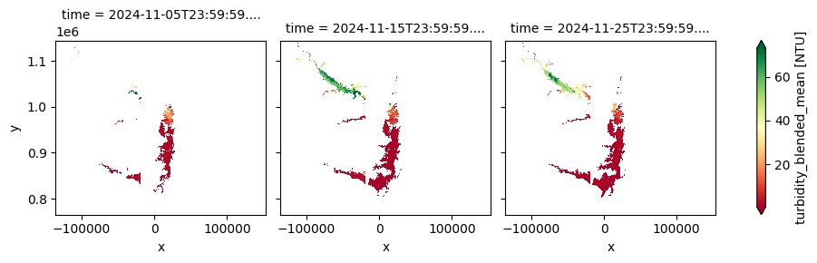
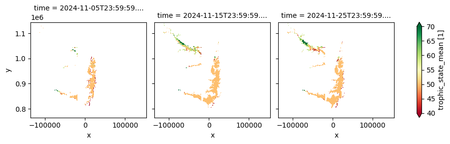
The dataset provides composites of key lake water quality parameters—such as turbidity, trophic state index, and surface reflectance—derived from Sentinel-2 MSI observations it is updated within four days after the end of each dekad. This version is designed for retrospective environmental monitoring and supports long-term assessment of lake ecosystem health and water clarity trends.
The cell below demonstrates how to load the dataset using the cgls_lwq100_2019_2024 product code for the Lake Water Quality 2019–2024 (100 m raster, 10-daily, version 1). Two measurements are loaded: trophic_state_mean and turbidity_blended_mean. Additional measurements and metadata can be found here. The most recent month of imagery is used in this example.
[5]:
#create reusable datacube query object
query = {
    'x': lons,
    'y': lats,
    'output_crs': 'epsg:6933',
}

#load the data
cgls_lwq100_2019_2024 = dc.load(product='cgls_lwq100_2019_2024',
                                measurements=['trophic_state_mean','turbidity_blended_mean'],
                                resolution = (-100, 100),
                                time = ('2024-11'),
                                **query)

# Mask no-data values
cgls_lwq100_2019_2024 = cgls_lwq100_2019_2024.where(cgls_lwq100_2019_2024 <= 996921)

#Display the xrray dataset
cgls_lwq100_2019_2024
[5]:
<xarray.Dataset> Size: 264MB
Dimensions:                 (time: 3, y: 3796, x: 2896)
Coordinates:
  * time                    (time) datetime64[ns] 24B 2024-11-05T23:59:59.500...
  * y                       (y) float64 30kB 1.145e+06 1.145e+06 ... 7.652e+05
  * x                       (x) float64 23kB -1.358e+05 -1.356e+05 ... 1.538e+05
    spatial_ref             int32 4B 6933
Data variables:
    trophic_state_mean      (time, y, x) float32 132MB nan nan nan ... nan nan
    turbidity_blended_mean  (time, y, x) float32 132MB nan nan nan ... nan nan
Attributes:
    crs:           epsg:6933
grid_mapping: spatial_refVisualizing the Results
[6]:
plt.figure(figsize=(15, 8))
cgls_lwq100_2019_2024['turbidity_blended_mean'].plot(col='time', cmap='RdYlGn', robust=True)
[6]:
<xarray.plot.facetgrid.FacetGrid at 0x7fe8280c7a40>
<Figure size 1500x800 with 0 Axes>
[7]:
plt.figure(figsize=(15, 8))
cgls_lwq100_2019_2024['trophic_state_mean'].plot(col='time',cmap='RdYlGn', robust=True)
[7]:
<xarray.plot.facetgrid.FacetGrid at 0x7fe8280c6330>
<Figure size 1500x800 with 0 Axes>
2. Lake Water Quality 2024 - present (raster 100 m), 10-daily – version 2
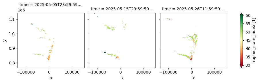
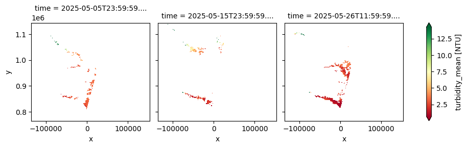
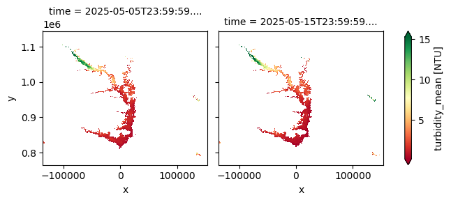
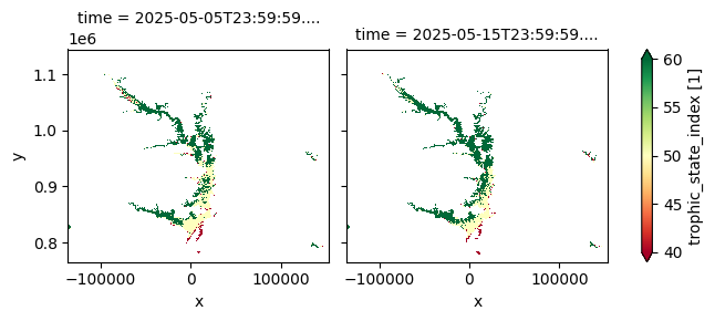
The dataset provides 10-day composites of key lake water quality parameters—including turbidity, chlorophyll‑a concentration, total suspended matter, and cyanobacteria risk—derived from Sentinel-2 MSI imagery at a 100 m resolution. It is designed to monitor the ecological condition of inland water bodies and support ongoing assessment of freshwater health. This second version introduces improved atmospheric correction, direct retrieval of turbidity from water-leaving reflectance, and additional quality flags to enhance the reliability of observations. With near-real-time updates available within three days after each dekad, the dataset supports environmental monitoring, water resource management, and early warning systems for water-related hazards across diverse lake systems.
The cell below demonstrates how to load the dataset using the cgls_lwq100_2024_nrt product code for the Lake Water Quality 2024 - present (100 m raster, 10-daily, version 1). Two measurements are loaded: trophic_state_index and turbidity_mean. Additional measurements and metadata can be found here. The most recent month of imagery is used in this example.
[8]:
#load the data
cgls_lwq100_2024_nrt = dc.load(product='cgls_lwq100_2024_nrt',
                                measurements=['trophic_state_index','turbidity_mean'],
                                resolution = (-100, 100),
                                time = ('2025-05'),
                                **query)

# Mask no-data values
cgls_lwq100_2024_nrt = cgls_lwq100_2024_nrt.where(cgls_lwq100_2024_nrt <= 996921)

cgls_lwq100_2024_nrt
[8]:
<xarray.Dataset> Size: 264MB
Dimensions:              (time: 3, y: 3796, x: 2896)
Coordinates:
  * time                 (time) datetime64[ns] 24B 2025-05-05T23:59:59.500000...
  * y                    (y) float64 30kB 1.145e+06 1.145e+06 ... 7.652e+05
  * x                    (x) float64 23kB -1.358e+05 -1.356e+05 ... 1.538e+05
    spatial_ref          int32 4B 6933
Data variables:
    trophic_state_index  (time, y, x) float32 132MB nan nan nan ... nan nan nan
    turbidity_mean       (time, y, x) float32 132MB nan nan nan ... nan nan nan
Attributes:
    crs:           epsg:6933
grid_mapping: spatial_refVisualizing the Results
[9]:
plt.figure(figsize=(15, 8))
cgls_lwq100_2024_nrt['trophic_state_index'].plot(col='time', cmap='RdYlGn', robust=True)
[9]:
<xarray.plot.facetgrid.FacetGrid at 0x7fe827e7dd60>
<Figure size 1500x800 with 0 Axes>
[10]:
plt.figure(figsize=(15, 8))
cgls_lwq100_2024_nrt['turbidity_mean'].plot(col='time', cmap='RdYlGn', robust=True)
[10]:
<xarray.plot.facetgrid.FacetGrid at 0x7fe827d82000>
<Figure size 1500x800 with 0 Axes>
3. Lake Water Quality 2002-2012 (raster 300 m), 10-daily – version 1
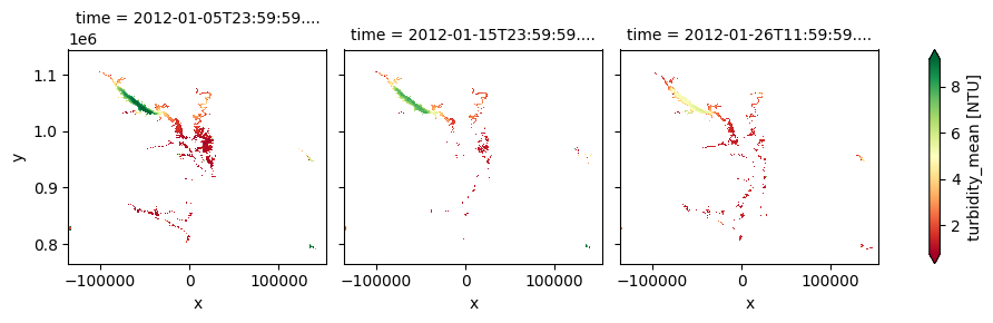
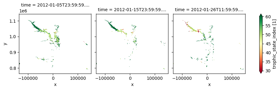
The dataset offers 10-day composites of lake water quality parameters—including turbidity, trophic state index, and surface reflectance—at a 300 m spatial resolution, derived from MERIS satellite observations. It enables historical assessments of lake ecosystem health and water clarity, making it particularly valuable for long-term monitoring and retrospective studies of medium to large lakes.
The cell below demonstrates how to load the dataset using the cgls_lwq300_2002_2012 product code for the Lake Water Quality 2024 - present (100 m raster, 10-daily, version 1). Two measurements are loaded: trophic_state_index and turbidity_mean. Additional measurements and metadata can be found here. The most recent month of imagery is used in this example.
[11]:
#load the data
cgls_lwq300_2002_2012 = dc.load(product='cgls_lwq300_2002_2012',
                                measurements=['trophic_state_index','turbidity_mean'],
                                resolution = (-300, 300),
                                time = ('2012-01'),
                                **query)

# Mask no-data values
cgls_lwq300_2002_2012 = cgls_lwq300_2002_2012.where(cgls_lwq300_2002_2012 <= 996921)

cgls_lwq300_2002_2012
[11]:
<xarray.Dataset> Size: 29MB
Dimensions:              (time: 3, y: 1265, x: 966)
Coordinates:
  * time                 (time) datetime64[ns] 24B 2012-01-05T23:59:59.500000...
  * y                    (y) float64 10kB 1.145e+06 1.144e+06 ... 7.654e+05
  * x                    (x) float64 8kB -1.358e+05 -1.354e+05 ... 1.538e+05
    spatial_ref          int32 4B 6933
Data variables:
    trophic_state_index  (time, y, x) float32 15MB nan nan nan ... nan nan nan
    turbidity_mean       (time, y, x) float32 15MB nan nan nan ... nan nan nan
Attributes:
    crs:           epsg:6933
grid_mapping: spatial_refVisualizing the Results
[12]:
plt.figure(figsize=(15, 8))
cgls_lwq300_2002_2012['turbidity_mean'].plot(col='time', cmap='RdYlGn', robust=True)
[12]:
<xarray.plot.facetgrid.FacetGrid at 0x7fe81d39e870>
<Figure size 1500x800 with 0 Axes>
[13]:
plt.figure(figsize=(15, 8))
cgls_lwq300_2002_2012['trophic_state_index'].plot(col='time', cmap='RdYlGn', robust=True)
[13]:
<xarray.plot.facetgrid.FacetGrid at 0x7fe8292beb40>
<Figure size 1500x800 with 0 Axes>
4. Lake Water Quality 2016-2024 (raster 300 m), 10-daily – version 1
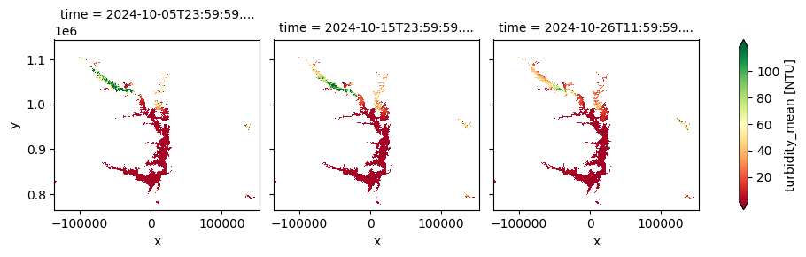
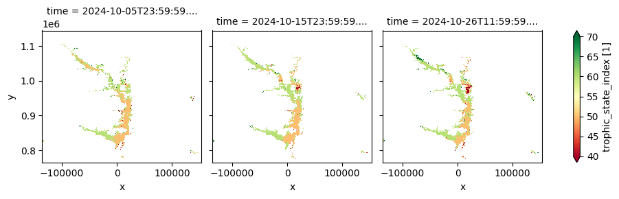
This product provides 10-day composites of key lake water quality parameters—including turbidity, trophic state index, and surface reflectance—at a 300 m spatial resolution, derived from Sentinel‑3 OLCI observations. Covering the period from April 30, 2016, to October 2024, it offers near-real-time updates within three days of each dekad and focuses on medium to large lakes. It is designed to support water quality monitoring, ecosystem health assessments, and environmental research.
The cell below demonstrates how to load the dataset using the cgls_lwq300_2016_2024 product code. Two measurements are loaded: trophic_state_index and turbidity_mean. Additional measurements and metadata can be found here. The most recent month of imagery is used in this example.
[14]:
#load the data
cgls_lwq300_2016_2024 = dc.load(product='cgls_lwq300_2016_2024',
                                measurements=['trophic_state_index','turbidity_mean'],
                                resolution = (-300, 300),
                                time = ('2024-10'),
                                **query)

# Mask no-data values
cgls_lwq300_2016_2024 = cgls_lwq300_2016_2024.where(cgls_lwq300_2016_2024 <= 996921)

cgls_lwq300_2016_2024
[14]:
<xarray.Dataset> Size: 29MB
Dimensions:              (time: 3, y: 1265, x: 966)
Coordinates:
  * time                 (time) datetime64[ns] 24B 2024-10-05T23:59:59.500000...
  * y                    (y) float64 10kB 1.145e+06 1.144e+06 ... 7.654e+05
  * x                    (x) float64 8kB -1.358e+05 -1.354e+05 ... 1.538e+05
    spatial_ref          int32 4B 6933
Data variables:
    trophic_state_index  (time, y, x) float32 15MB nan nan nan ... nan nan nan
    turbidity_mean       (time, y, x) float32 15MB nan nan nan ... nan nan nan
Attributes:
    crs:           epsg:6933
grid_mapping: spatial_refVisualizing the Results
[15]:
plt.figure(figsize=(15, 8))
cgls_lwq300_2016_2024['turbidity_mean'].plot(col='time', cmap='RdYlGn', robust=True)
[15]:
<xarray.plot.facetgrid.FacetGrid at 0x7fe825406a80>
<Figure size 1500x800 with 0 Axes>
[16]:
plt.figure(figsize=(15, 8))
cgls_lwq300_2016_2024['trophic_state_index'].plot(col='time', cmap='RdYlGn', robust=True)
[16]:
<xarray.plot.facetgrid.FacetGrid at 0x7fe81d39f860>
<Figure size 1500x800 with 0 Axes>
5. Lake Water Quality 2024 - present (raster 300 m), 10-daily – version 2
The Lake Water Quality 2024–present dataset offers 10-day composites of key water quality parameters at a 300 m spatial resolution, based on Sentinel-3 OLCI observations. Version 2 expands the dataset by including additional indicators—such as chlorophyll‑a concentration, total suspended matter, cyanobacteria risk, and quality flags. Designed for near-real-time freshwater monitoring, it is updated within three days of each dekad, supporting timely assessments of water clarity and biological activity in lakes.
The cell below demonstrates how to load the dataset using the cgls_lwq300_2024_nrt product code. Two measurements are loaded: trophic_state_index and turbidity_mean. Additional measurements and metadata can be found here. The most recent month of imagery is used in this example.
[17]:
#load the data
cgls_lwq300_2024_nrt = dc.load(product='cgls_lwq300_2024_nrt',
                                measurements=['trophic_state_index','turbidity_mean'],
                                resolution = (-300, 300),
                                time = ('2025-05'),
                                **query)

# Mask no-data values
cgls_lwq300_2024_nrt = cgls_lwq300_2024_nrt.where(cgls_lwq300_2024_nrt <= 996921)

cgls_lwq300_2024_nrt
[17]:
<xarray.Dataset> Size: 20MB
Dimensions:              (time: 2, y: 1265, x: 966)
Coordinates:
  * time                 (time) datetime64[ns] 16B 2025-05-05T23:59:59.500000...
  * y                    (y) float64 10kB 1.145e+06 1.144e+06 ... 7.654e+05
  * x                    (x) float64 8kB -1.358e+05 -1.354e+05 ... 1.538e+05
    spatial_ref          int32 4B 6933
Data variables:
    trophic_state_index  (time, y, x) float32 10MB nan nan nan ... nan nan nan
    turbidity_mean       (time, y, x) float32 10MB nan nan nan ... nan nan nan
Attributes:
    crs:           epsg:6933
grid_mapping: spatial_refVisualizing the Results
[18]:
plt.figure(figsize=(15, 8))
cgls_lwq300_2024_nrt['turbidity_mean'].plot(col='time', cmap='RdYlGn', robust=True)
[18]:
<xarray.plot.facetgrid.FacetGrid at 0x7fe8250d4fb0>
<Figure size 1500x800 with 0 Axes>
[19]:
plt.figure(figsize=(15, 8))
cgls_lwq300_2024_nrt['trophic_state_index'].plot(col='time', cmap='RdYlGn', robust=True)
[19]:
<xarray.plot.facetgrid.FacetGrid at 0x7fe8250d4e30>
<Figure size 1500x800 with 0 Axes>
Conclusion
This notebook demonstrates how to load the lake water quality dataset in the DE Africa Sandbox. Beyond this initial step, further analysis can be performed to extract deeper insights into lake conditions and ecosystem dynamics. These include time-series analysis to monitor seasonal trends, anomaly detection to identify unusual events (e.g., algal blooms), and spatial comparison across lakes. The dataset can also be combined with rainfall, land cover, population density, or catchment land use data to explore potential drivers of water quality change, and to identify and compare water quality across lakes in different regions or climatic zones, enabling a better understanding of spatial variability.
References
Copernicus Land Monitoring Service. (2024). Lake Water Quality v2.0 (100 m), global, 10-daily – 2024–present. Retrieved from https://land.copernicus.eu/en/products/water-bodies/lake-water-quality-v2-0-100m
Copernicus Land Monitoring Service. (2024). Lake Water Quality Near Real-Time v2.0 (300 m), global, 10-daily – 2024–present. Retrieved from https://land.copernicus.eu/en/products/water-bodies/lake-water-quality-near-real-time-v2-0-300m
Copernicus Land Monitoring Service. (2019). Lake Water Quality v1.0 (100 m), global, 10-daily – 2019–2024. Retrieved from https://land.copernicus.eu/en/products/water-bodies/lake-water-quality-v1-0-100m
Copernicus Land Monitoring Service. (2016). Lake Water Quality Near Real-Time v1.0 (300 m), global, 10-daily – 2016–2024. Retrieved from https://land.copernicus.eu/en/products/water-bodies/lake-water-quality-near-real-time-v1-0-300m
Copernicus Land Monitoring Service. (2002). Lake Water Quality Offline v1.0 (300 m), global, 10-daily – 2002–2012. Retrieved from https://land.copernicus.eu/en/products/water-bodies/lake-water-quality-offline-v1-0-300m
Additional information
License: The code in this notebook is licensed under the Apache License, Version 2.0. Digital Earth Africa data is licensed under the Creative Commons by Attribution 4.0 license.
Contact: If you need assistance, please post a question on the Open Data Cube Slack channel or on the GIS Stack Exchange using the open-data-cube tag (you can view previously asked questions here). If you would like to report an issue with this notebook, you can file one on
Github.
Compatible datacube version:
[20]:
print(datacube.__version__)
1.8.20
Last tested:
[21]:
from datetime import datetime
datetime.today().strftime('%Y-%m-%d')
[21]:
'2025-06-18'