Cropland extent maps for Africa
Products used: crop_mask
Keywords: datasets; crop_mask, analysis; agriculture, cropland extent
Background
A central focus for governing bodies in Africa is the need to secure the necessary food sources to support their populations. It has been estimated that the current production of crops will need to double by 2050 to meet future needs for food production. Higher level crop-based products that can assist with managing food insecurity, such as cropping watering intensities, crop types, or crop productivity, require as a starting point precise and accurate cropland extent maps indicating where cropland occurs. Current cropland extent maps are either inaccurate, have coarse spatial resolutions, or are not updated regularly. An accurate, high-resolution, and regularly updated cropland area map for the African continent is therefore recognised as a gap in the current crop monitoring services.
Digital Earth Africa’s cropland extent maps for Africa show the estimated location of croplands for the period of January to Decemeber 2019.
For a full description of the product specifications, validation results, and methods used to develop the products, see the Cropland_extent_specifications document.
Description
This notebook will show you how to load, plot, and conduct a simple analysis using the cropland extent product. The steps are as follows:
List the available cropland extent products
Load the
crop_maskproductPlotting the different measurements of the crop-mask
Example analysis 1: Identifying crop trends with NDVI
Example analysis 2: Comparison of cropped area with global land cover datasets
Inspect different regions of the crop mask.
For a more detailed example of using the cropland extent product, see the following notebooks:
Getting started
To run this analysis, run all the cells in the notebook, starting with the “Load packages” cell.
Load packages
Import Python packages that are used for the analysis.
[1]:
%matplotlib inline

import datacube
import xarray as xr
import matplotlib.pyplot as plt

from deafrica_tools.plotting import display_map
from deafrica_tools.bandindices import calculate_indices
from deafrica_tools.datahandling import load_ard
Connect to the datacube
Connect to the datacube so we can access DE Africa data.
[2]:
dc = datacube.Datacube(app='cropland_extent')
Analysis parameters
This section defines the analysis parameters, including:
lat, lon, buffer: center lat/lon and analysis window size for the area of interesttime_period: time period to load for the crop mask. Currently, only a map for 2019 is availableresolution: the pixel resolution to use for loading thecrop_mask_<region>. The native resolution of the product is 10 metres i.e.(-10,10)
The default location is in a extensivley cultivated valley north of Addis Ababa, Ethiopia
[3]:
lat, lon = 8.5615, 40.691

buffer = 0.04

time_period = ('2019')

resolution=(-10, 10)

#join lat, lon, buffer to get bounding box
lon_range = (lon - buffer, lon + buffer)
lat_range = (lat + buffer, lat - buffer)
View the selected location
The next cell will display the selected area on an interactive map. Feel free to zoom in and out to get a better understanding of the area you’ll be analysing. Clicking on any point of the map will reveal the latitude and longitude coordinates of that point.
[4]:
display_map(lon_range, lat_range)
[4]:
List cropland extent products available in Digital Earth Africa
We can use datacube’s list_measurements functionality to inspect the cropland extent products available in the datacube. The table below shows the product names you can use to load data, and the measurements available for each product. The cropland extent masks come with three measurements: mask, filtered, and prob.
We can see in the table below that there is a single crop_mask product which covers the entire continent. It is comprised of numerous crop_mask_<region> products stitched together. We can use the continental crop_mask products for most applications, though we should be aware of the boundaries of the regional products that comprise it. We will explore this further below.
[5]:
dc_measurements = dc.list_measurements()
dc_measurements.filter(like='crop_mask', axis=0)
[5]:
| name | dtype | units | nodata | aliases | flags_definition | ||
|---|---|---|---|---|---|---|---|
| product | measurement | ||||||
| crop_mask | mask | mask | uint8 | 1 | 255.0 | [crop_mask, MASK] | NaN |
| prob | prob | uint8 | 1 | 255.0 | [crop_prob, PROB] | NaN | |
| filtered | filtered | uint8 | 1 | 255.0 | [mode] | NaN | |
| crop_mask_central | mask | mask | uint8 | 1 | 0.0 | [crop_mask, MASK] | NaN |
| prob | prob | uint8 | 1 | 0.0 | [crop_prob, PROB] | NaN | |
| filtered | filtered | uint8 | 1 | 0.0 | [mode] | NaN | |
| crop_mask_eastern | mask | mask | uint8 | 1 | 0.0 | [crop_mask, MASK] | NaN |
| prob | prob | uint8 | 1 | 0.0 | [crop_prob, PROB] | NaN | |
| filtered | filtered | uint8 | 1 | 0.0 | [mode] | NaN | |
| crop_mask_indian_ocean | mask | mask | uint8 | 1 | 0.0 | [crop_mask, MASK] | NaN |
| prob | prob | uint8 | 1 | 0.0 | [crop_prob, PROB] | NaN | |
| filtered | filtered | uint8 | 1 | 0.0 | [mode] | NaN | |
| crop_mask_northern | mask | mask | uint8 | 1 | 0.0 | [crop_mask, MASK] | NaN |
| prob | prob | uint8 | 1 | 0.0 | [crop_prob, PROB] | NaN | |
| filtered | filtered | uint8 | 1 | 0.0 | [mode] | NaN | |
| crop_mask_sahel | mask | mask | uint8 | 1 | 0.0 | [crop_mask, MASK] | NaN |
| prob | prob | uint8 | 1 | 0.0 | [crop_prob, PROB] | NaN | |
| filtered | filtered | uint8 | 1 | 0.0 | [mode] | NaN | |
| crop_mask_southeast | mask | mask | uint8 | 1 | 0.0 | [crop_mask, MASK] | NaN |
| prob | prob | uint8 | 1 | 0.0 | [crop_prob, PROB] | NaN | |
| filtered | filtered | uint8 | 1 | 0.0 | [mode] | NaN | |
| crop_mask_southern | mask | mask | uint8 | 1 | 0.0 | [crop_mask, MASK] | NaN |
| prob | prob | uint8 | 1 | 0.0 | [crop_prob, PROB] | NaN | |
| filtered | filtered | uint8 | 1 | 0.0 | [mode] | NaN | |
| crop_mask_western | mask | mask | uint8 | 1 | 0.0 | [crop_mask, MASK] | NaN |
| prob | prob | uint8 | 1 | 0.0 | [crop_prob, PROB] | NaN | |
| filtered | filtered | uint8 | 1 | 0.0 | [mode] | NaN |
Loading the cropland extent product
In this example, we will load the 'crop_mask' product.
[6]:
# generate a query object from the analysis parameters
query = {
    'time': time_period,
    'x': lon_range,
    'y': lat_range,
    'resolution':resolution
}

# now load the crop-mask using the query
cm = dc.load(product='crop_mask',
             **query).squeeze()
print(cm)
<xarray.Dataset> Size: 2MB
Dimensions:      (y: 1011, x: 773)
Coordinates:
    time         datetime64[ns] 8B 2019-07-02T11:59:59.999999
  * y            (y) float64 8kB 1.093e+06 1.093e+06 ... 1.083e+06 1.083e+06
  * x            (x) float64 6kB 3.922e+06 3.922e+06 ... 3.93e+06 3.93e+06
    spatial_ref  int32 4B 6933
Data variables:
    mask         (y, x) uint8 782kB 0 0 0 0 0 0 0 0 0 0 ... 0 0 0 0 0 0 0 0 0 0
    prob         (y, x) uint8 782kB 41 41 41 45 43 45 40 ... 17 18 24 22 23 22
    filtered     (y, x) uint8 782kB 0 0 0 0 0 0 0 0 0 0 ... 0 0 0 0 0 0 0 0 0 0
Attributes:
    crs:           epsg:6933
    grid_mapping:  spatial_ref
Plotting the cropland extent
Above, we can see the crop_mask products contains three measurements:
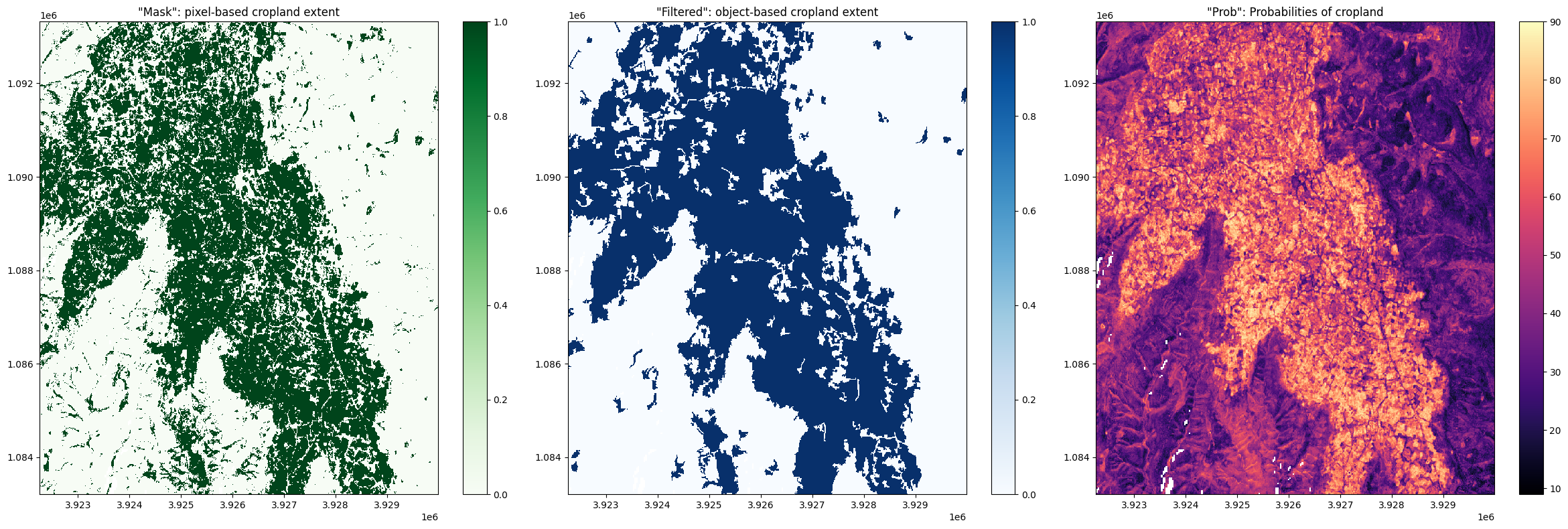
mask: This band displays cropped regions as a binary map. Values of1indicate the presence of crops, while a value of0indicates the absence of cropping. This band is a pixel-based cropland extent map, meaning the map displays the raw output of the pixel-based Random Forest classification.prob: This band displays the prediction probabilities for the ‘crop’ class. As this service uses a random forest classifier, the prediction probabilities refer to the percentage of trees that voted for the random forest classification. For example, if the model had 200 decision trees in the random forest, and 150 of the trees voted ‘crop’, the prediction probability is 150 / 200 x 100 = 75 %. Thresholding this band at > 50 % will produce a map identical tomask.filtered: This band displays cropped regions as a binary map. Values of1indicate the presence of crops, while a value of0indicates the absence of cropping. This band is an object-based cropland extent map where themaskband has been filtered using an image segmentation algorithm (see this paper for details on the algorithm used). During this process, segments smaller than 1 Ha (100 10m x 10m pixels) are merged with neighbouring segments, resulting in a map where the smallest classified region is 1 Ha in size. Thefiltereddataset is provided as a complement to themaskband; small commission errors are removed by object-based filtering, and the ‘salt and pepper’ effect typical of classifying pixels is diminished.
Below, we will plot the three measurements side-by-side:
[7]:
fig, axes = plt.subplots(1, 3, figsize=(24, 8))
cm.mask.where(cm.mask<255).plot(ax=axes[0], # we filter to <255 to omit missing data
                   cmap='Greens',
                   add_labels=False)

cm.filtered.where(cm.filtered<255).plot(ax=axes[1],
                   cmap='Blues',
                   add_labels=False)

cm.prob.where(cm.prob<255).plot(ax=axes[2],
                   cmap='magma',
                   add_labels=False)

axes[0].set_title('"Mask": pixel-based cropland extent')
axes[1].set_title('"Filtered": object-based cropland extent')
axes[2].set_title('"Prob": Probabilities of cropland');

plt.tight_layout();
Example application: Identifying crop trends with NDVI
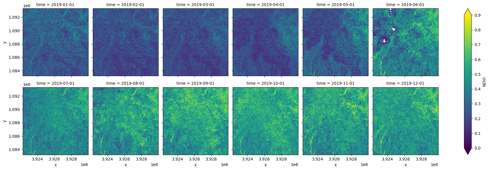
The Normalised Difference Vegetation Index (NDVI) can be used to track the health and growth of crops as they mature. Here will load an annual time series of Sentinel-2 satellite data, calculate the NDVI, and mask the region with DE Africa’s cropland extent product. With only the cropping pixels remaining, we can summarise the growth cycle of the crops within the region.
[8]:
ds = load_ard(dc=dc,
              products=['s2_l2a'],
              time=('2019-01', '2019-12'),
              measurements=['red', 'nir'],
              mask_filters=(['opening',5],['closing', 5]), #improve cloud mask
              min_gooddata=0.35,
              like=cm.geobox
             )
Using pixel quality parameters for Sentinel 2
Finding datasets
    s2_l2a
Counting good quality pixels for each time step
/opt/venv/lib/python3.10/site-packages/rasterio/warp.py:387: NotGeoreferencedWarning: Dataset has no geotransform, gcps, or rpcs. The identity matrix will be returned.
  dest = _reproject(
Filtering to 122 out of 158 time steps with at least 35.0% good quality pixels
Applying morphological filters to pq mask (['opening', 5], ['closing', 5])
Applying pixel quality/cloud mask
Loading 122 time steps
Calculate NDVI
[9]:
ds = calculate_indices(ds, 'NDVI', drop=True, satellite_mission='s2')
Dropping bands ['red', 'nir']
Resample the dataset to monthly time-steps
[10]:
ds = ds.NDVI.resample(time='MS').mean()

#plot the result
ds.plot.imshow(col='time', col_wrap=6, vmin=0, vmax=0.9);
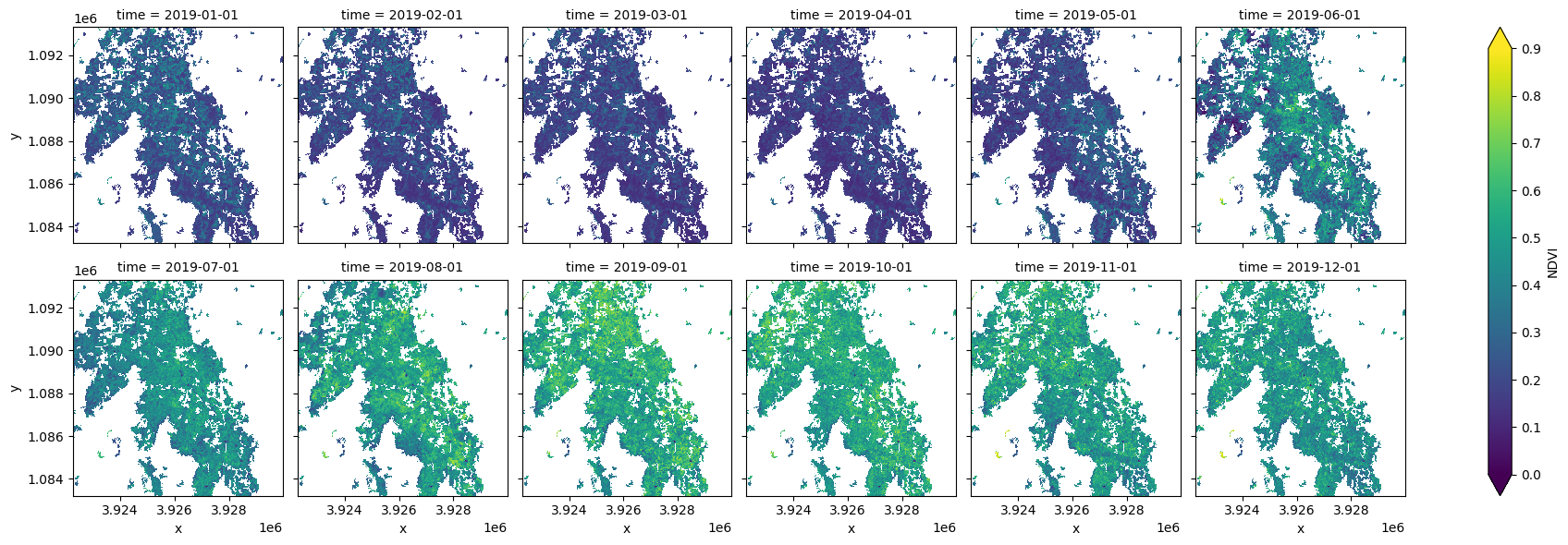
Mask with the cropland extent map
Using the measurement filtered, we can mask the dataset with the crop_mask product.
[11]:
#Filter out the no-data pixels (255) and non-crop pixels (0) from the crop-mask 'filtered' band and
#mask using 'filtered' band.
ds = ds.where(cm.filtered == 1)

ds.plot.imshow(col='time', col_wrap=6, vmin=0, vmax=0.9);
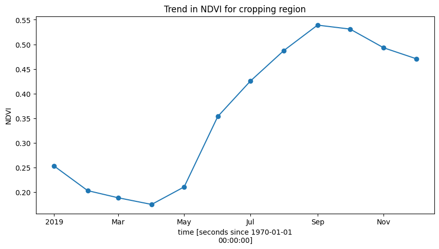
Summarise the trends in NDVI for the croppping regions with a line plot
Below, the plot shows the cropping schedule starts in April, with the peak of the growing season occuring towards the end of the year in October/November.
[12]:
ds.mean(['x', 'y']).plot.line(marker='o', figsize=(10,5))
plt.title('Trend in NDVI for cropping region');
Example Analysis 2: Comparison with global landcover datasets
Indexed within the DE Africa’s datacube are two global 10m resolution landcover datasets that each contain a cropping class. These landcover datasets were both produced using Senitnel-2 images, the same as DE Afric’s cropland extent product. Below, we will load the landcover datasets over the same region as the cropland extent map and compare the area classified as croppping. You can use the interactive map plotted below to determine the areas where each datasets does well (or poorly) at classifying crops.
To learn more about the landcover datasets see the Landcover Classification notebook.
First, we need to re-enter some analysis parameters. You’ll notice below we’ve set the resolution to 60m to allow us to load a large region quickly, though all datasets are natively stored at 10m resolution.
The default region is a bounding box over Lake Kyoga, Uganda. This region is extensively cropped.
[13]:
lat, lon = 1.4315, 33.1207

buffer = 1.0

resolution=(-60, 60) #resample to load larger area

#join lat, lon, buffer to get bounding box
lon_range = (lon - buffer, lon + buffer)
lat_range = (lat + buffer, lat - buffer)
Plot an interactive map
If you zoom in you can examine the dominant land cover classes in the region (hint, there’s a lot of agriculture!)
[14]:
display_map(lon_range, lat_range)
[14]:
Load the cropland extent, ESRI’s Landcover product, and ESA’s WorldCover product
[15]:
# generate a query object from the analysis parameters
query = {
    'x': lon_range,
    'y': lat_range,
    'resolution':resolution
}

# now load the crop-mask using the query
cm = dc.load(product='crop_mask', measurements=['mask'], **query, time='2019').squeeze()

#load the two landcover datasets for the year 2020.
lulc_esa = dc.load(product='esa_worldcover_2020', time="2020", measurements='classification', like=cm.geobox).squeeze()
lulc_esri = dc.load(product='io_lulc_v2', time="2020-07", measurements='classification', like=cm.geobox).squeeze()
Reclassify the landcover datasets to a binary crop/non-crop image to allow a straightforward comparison with DE Africa’s cropland extent map
[16]:
esri_crops = xr.where(lulc_esri['classification']==5, 1, 0)
esa_crops = xr.where(lulc_esa['classification']==40, 1, 0)
Filter out the no-data pixels (255) from the crop-mask mask band.
[17]:
cm_mask = cm.mask.where(cm.mask != 255)
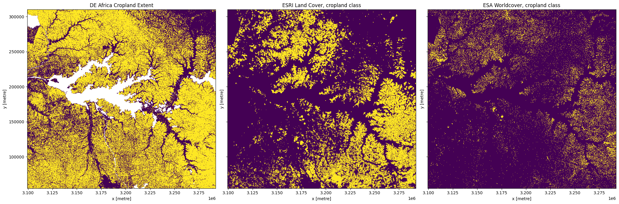
Plot the cropping extent of the three datasets
[18]:
fig,ax=plt.subplots(1,3, sharey=True, figsize=(21,7))
cm_mask.plot.imshow(ax=ax[0], add_colorbar=False)
esri_crops.plot.imshow(ax=ax[1], add_colorbar=False)
esa_crops.plot.imshow(ax=ax[2], add_colorbar=False)
ax[0].set_title('DE Africa Cropland Extent')
ax[1].set_title('ESRI Land Cover, cropland class')
ax[2].set_title('ESA Worldcover, cropland class')
plt.tight_layout();
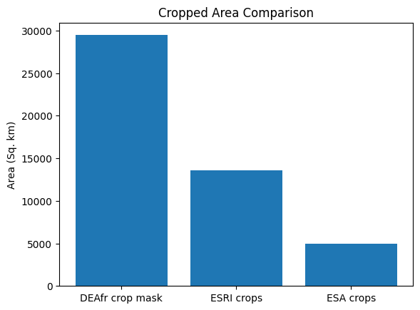
Calculate the cropped area in each product
In this example, you’ll see that DE Africa’s cropland product maps a lot more cropping than the two global landcover products. In this example, the DE Africa product is more accurate than the landcover datasets. However, over wetlands in the south-west of Lake Kyoga DE Afria’s product incorrectly maps some of the wetlands as cropping, while the landcover datasets do not. While there are regions where DE AFrica’s cropland extent maps have errors, in general they are much more accurate than any of the currently existing landcover datasets over Africa.
[19]:
pixel_length = query["resolution"][1]
m_per_km = 1000  # conversion from metres to kilometres
area_per_pixel = pixel_length**2 / m_per_km**2
[20]:
cm_area = cm_mask.sum().data * area_per_pixel
esri_area = esri_crops.sum().data * area_per_pixel
esa_area = esa_crops.sum().data * area_per_pixel

label = ['DEAfr crop mask', 'ESRI crops', 'ESA crops']
plt.bar(label, [cm_area,esri_area,esa_area])
plt.ylabel("Area (Sq. km)")
plt.title('Cropped Area Comparison');
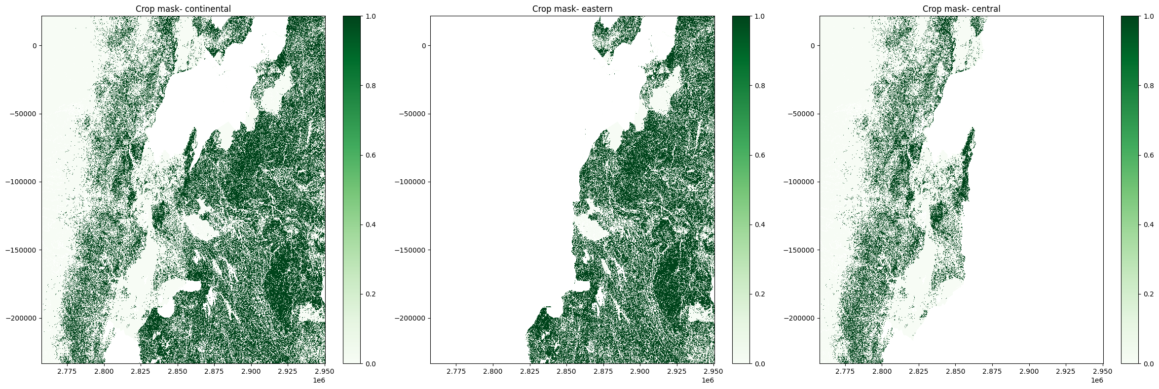
Regional crop mask boundaries
As we saw in the datasets table, the crop_mask is comprised of numerous regional products stitched together. We can load and use the continental crop_mask product for most applications. However, we may observe some unusual artefacts at the boundaries of regional crop masks which are worth being aware of. We will investigate this below.
First, we will define and inspect an area on the borders of Uganda, Rwanda, and DR Congo. This also forms the border the crop_mask_central and crop_mask_eastern. We can inspect the extent of each regional product on the Digital Earth Africa Maps Platform.
[21]:
lat, lon = -0.83, 29.58

buffer = 1.0

resolution=(-60, 60) #resample to load larger area

#join lat, lon, buffer to get bounding box
lon_range = (lon - buffer, lon + buffer)
lat_range = (lat + buffer, lat - buffer)
[22]:
display_map(lon_range, lat_range)
[22]:
[23]:
query = {
    'x': lon_range,
    'y': lat_range,
    'resolution':resolution
}
Load regional crop masks
Below, we load the continental product in addtion to both the central and eastern crop masks. We do this by using the region argument in dc.load.
[24]:
cm = dc.load(product='crop_mask',
             measurements=['mask'],
             time='2019',
             **query).squeeze()

cm_east = dc.load(
             product='crop_mask',
             region='eastern',
             measurements=['mask'],
             time='2019',
             **query).squeeze()

cm_central = dc.load(
             product='crop_mask',
             region='central',
             measurements=['mask'],
             time='2019',
             **query).squeeze()
Plot regional products
[25]:
fig, axes = plt.subplots(1, 3, figsize=(24, 8))
cm.mask.where(cm.mask<255).plot(ax=axes[0], # we filter to <255 to omit missing data
                   cmap='Greens',
                   add_labels=False)

cm_east.mask.where(cm_east.mask<255).plot(ax=axes[1],
                   cmap='Greens',
                   add_labels=False)

cm_central.mask.where(cm_central.mask<255).plot(ax=axes[2],
                   cmap='Greens',
                   add_labels=False)

axes[0].set_title('Crop mask- continental')
axes[1].set_title('Crop mask- eastern')
axes[2].set_title('Crop mask- central');

plt.tight_layout();
Additional information
License: The code in this notebook is licensed under the Apache License, Version 2.0. Digital Earth Africa data is licensed under the Creative Commons by Attribution 4.0 license.
Contact: If you need assistance, please post a question on the Open Data Cube Slack channel or on the GIS Stack Exchange using the open-data-cube tag (you can view previously asked questions here). If you would like to repoart an issue with this notebook, you can file one on
Github.
Compatible datacube version:
[26]:
print(datacube.__version__)
1.8.19
Last Tested:
[27]:
from datetime import datetime
datetime.today().strftime('%Y-%m-%d')
[27]:
'2024-11-22'