Monthly NDVI Anomaly

• Products used: ndvi_anomaly, crop_mask

Keywords: data datasets; ndvi anomaly, data used; crop_mask

Background

Digital Earth Africa’s Monthly NDVI and Anomalies service provides an estimate of vegetation condition for each calendar month, as well as comparison of this against the long-term baseline condition measured for the month over the period 1984 to 2020 in the NDVI Climatology.

A standardised anomaly is calculated by subtracting the long-term mean from an observation of interest and then dividing the result by the long-term standard deviation. The equation below applies for monthly NDVI anomalies:

\begin{equation} \text{Standardised anomaly }=\frac{\text{NDVI}_{month, year}-\text{NDVI}_{month}}{\sigma} \end{equation}

where \(\text{NDVI}_{month, year}\) is the NDVI measured for a month in a year, \(\text{NDVI}_{month}\) is the long-term mean for this month from 1984 to 2020, and \(\sigma\) is the long-term standard deviation. A standarised anomaly therefore measures the direction and significance of vegetation change against normal conditions.

Positive NDVI anomaly values indicate vegetation is greener than average conditions, and are usually due to increased rainfall in a region. Negative values indicate additional plant stress relative to the long-term average. The NDVI anomaly service is therefore effective for understanding the extent, intensity and impact of a drought.

Abrupt and significant negative anomalies may also be caused by fire disturbance.

Further details on the product are available in the NDVI Anomaly technical specifications documentation.

Important details:

• Datacube product name: ndvi_anomaly

• Measurements

  • ndvi_mean: Mean NDVI for a month.

  • ndvi_std_anomaly: Standardised NDVI anomaly for a month

  • clear_count: Number of clear observations in a month

• Date-range: monthly from January 2017

• Spatial resolution: 30m

From September 2022, the Monthly NDVI Anomaly is generated as a low latency product, i.e. anomaly for a month is generated on the 5th day of the following month. This ensures data is available shortly after the end of a month and all Landsat 9 and Sentinel-2 observations are included. Not all Landsat 8 observations for the month will be used, because the Landsat 8 Surface Refelectance product from USGS has a latency of over 2 weeks (see Landsat Collection 2 Generation Timeline).

From January 2017 to August 2022, all available Landsat 8, Landsat 9 and Sentinel-2 observations are used in the calculation of the anomalies.

Description

In this notebook we will load the NDVI and Anomalies product using dc.load() to return the mean, standard deviation, and clear observation count for each calendar month. A final section explores an example analysis using the product.

Topics covered include:

1. Inspecting the NDVI and Anomalies product and measurements available in the datacube.

2. Using the native dc.load() function to load in NDVI Anomaly for a defined area.

3. Visualise the mean NDVI and standardised anomalies.

4. Plot the phenology curve of croplands.

5. Extract mean NDVI and anomalies for a selected month and region.

6. Compare mean NDVI to conditions observed in the previous years.

---

Getting started

To run this analysis, run all the cells in the notebook, starting with the “Load packages” cell.

Load packages

import datacube
import numpy as np
import xarray as xr
import pandas as pd
import geopandas as gpd
import matplotlib as mpl
import matplotlib.pyplot as plt
import matplotlib.dates as mdates
from matplotlib.colors import ListedColormap
from odc.ui import with_ui_cbk
from odc.geo.geom import Geometry

from deafrica_tools.plotting import display_map
from deafrica_tools.spatial import xr_rasterize

Connect to the datacube

dc = datacube.Datacube(app='NDVI_anomaly')

Available measurements

List measurements

The table printed below shows the measurements available in the NDVI and Anomalies product. The mean NDVI, standardised NDVI anomaly, and clear obervations count can be loaded for each calendar month.

product_name = 'ndvi_anomaly'

dc_measurements = dc.list_measurements()
dc_measurements.loc[product_name].drop('flags_definition', axis=1)

	name	dtype	units	nodata	aliases	scale_factor
measurement
ndvi_mean	ndvi_mean	float32	1	NaN	[NDVI_MEAN]	NaN
ndvi_std_anomaly	ndvi_std_anomaly	float32	1	NaN	[NDVI_STD_ANOMALY]	NaN
clear_count	clear_count	int8	1	0.0	[CLEAR_COUNT, count]	NaN

Analysis parameters

This section defines the analysis parameters, including:

• lat, lon, buffer: center lat/lon and analysis window size for the area of interest.

• resolution: the pixel resolution to use for loading the ndvi_anomaly. The native resolution of the product is 30 metres i.e. (-30,30) as the product is Landsat derived.

• time_range: time range for loading the monthly anomalies.

The default location is a cropping region in Western Cape, South Africa where an irrigation scheme along a river is surrounded by rain-fed cropping.

lat, lon = -34.0602, 20.2800  # capetown

buffer = 0.08

resolution = (-30, 30)

# join lat, lon, buffer to get bounding box
lon_range = (lon - buffer, lon + buffer)
lat_range = (lat + buffer, lat - buffer)

time = '2020'

View the selected location

The next cell will display the selected area on an interactive map. Feel free to zoom in and out to get a better understanding of the area you’ll be analysing. Clicking on any point of the map will reveal the latitude and longitude coordinates of that point.

display_map(lon_range, lat_range)

Make this Notebook Trusted to load map: File -> Trust Notebook

Load data

Below, we use the dc.load function to load all the measurements over the region specified above.

# load data
ndvi_anom = dc.load(
    product="ndvi_anomaly",
    resolution=resolution,
    x=lon_range,
    y=lat_range,
    time=time,
    progress_cbk=with_ui_cbk(),
)

print(ndvi_anom)

<xarray.Dataset> Size: 32MB
Dimensions:           (time: 12, y: 567, x: 515)
Coordinates:
  * time              (time) datetime64[ns] 96B 2020-01-16T11:59:59.999999 .....
  * y                 (y) float64 5kB -4.091e+06 -4.091e+06 ... -4.108e+06
  * x                 (x) float64 4kB 1.949e+06 1.949e+06 ... 1.964e+06
    spatial_ref       int32 4B 6933
Data variables:
    ndvi_mean         (time, y, x) float32 14MB 0.4438 0.4615 ... 0.1562 0.1542
    ndvi_std_anomaly  (time, y, x) float32 14MB -0.3588 0.2575 ... -0.7113
    clear_count       (time, y, x) int8 4MB 10 11 11 11 11 11 ... 12 12 12 12 12
Attributes:
    crs:           epsg:6933
    grid_mapping:  spatial_ref

Plotting monthly NDVI and anomalies

# define  colormaps for NDVI STD Anomalies
top = mpl.colormaps['copper'].resampled(128)
bottom = mpl.colormaps['Greens'].resampled(128)
# create a new colormaps with a name of BrownGreen
newcolors = np.vstack((top(np.linspace(0, 1, 128)),
                       bottom(np.linspace(0, 1, 128))))
cramp = ListedColormap(newcolors, name='cramp')

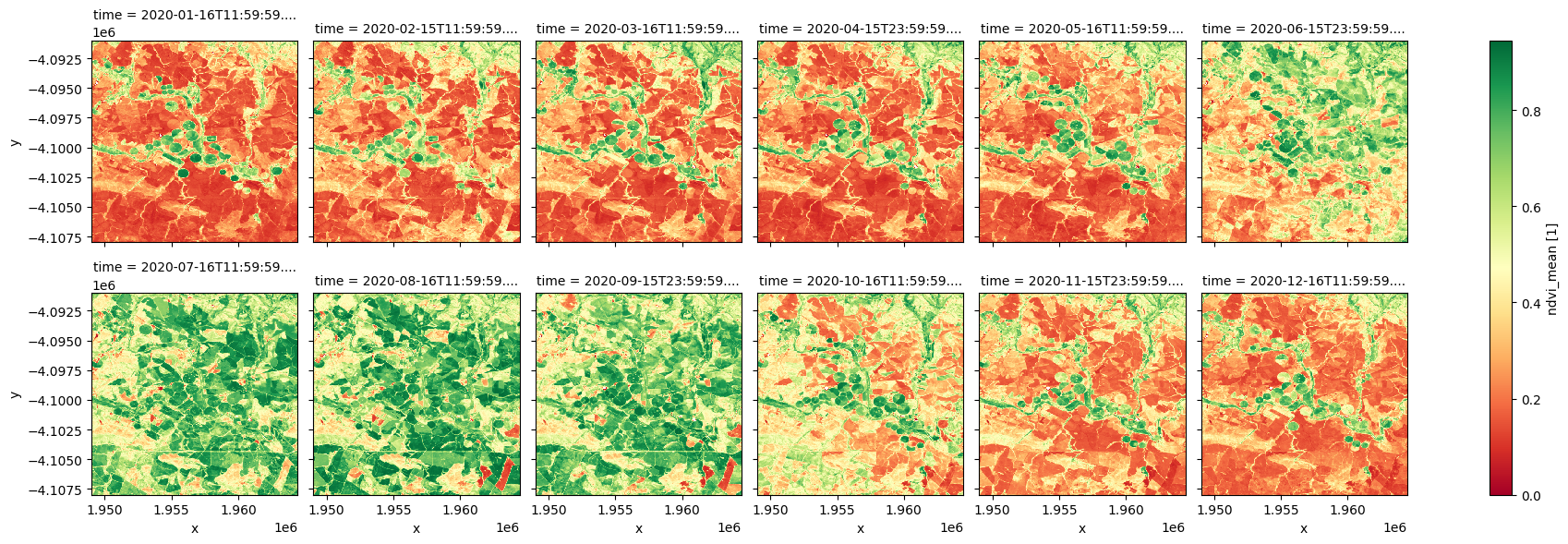
ndvi_anom.ndvi_mean.plot.imshow(col='time', col_wrap=6, cmap="RdYlGn");

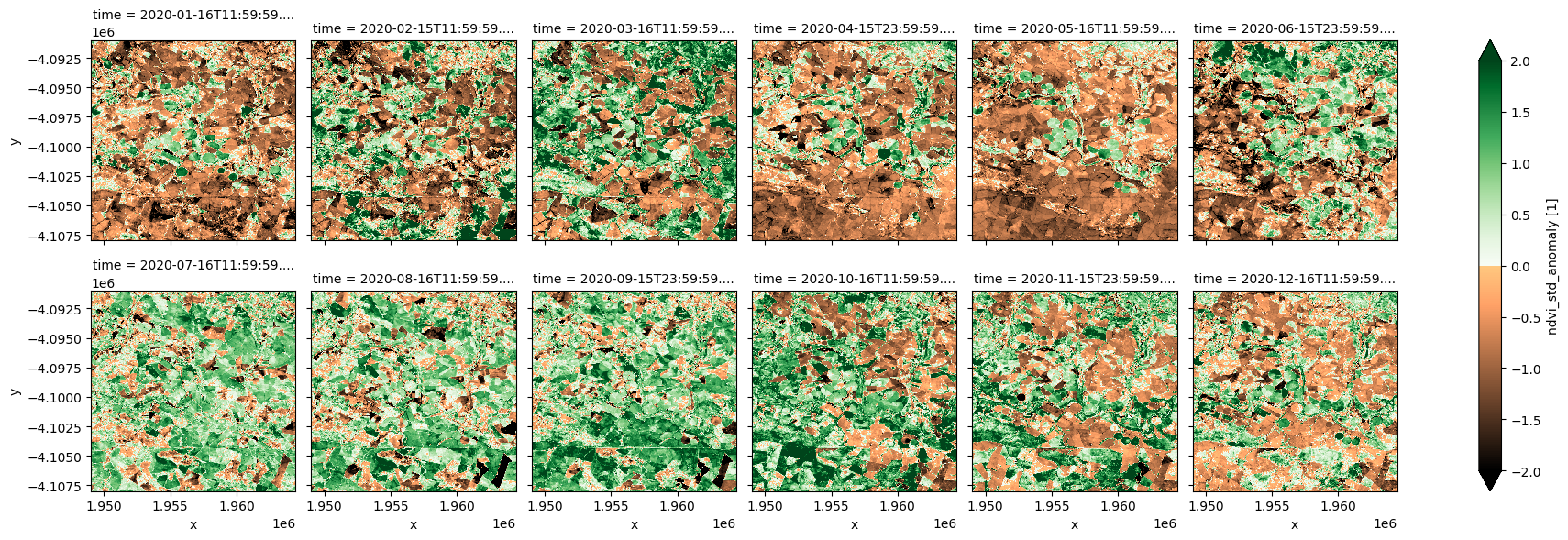
ndvi_anom.ndvi_std_anomaly.plot.imshow(col='time', col_wrap=6, cmap=cramp, vmin=-2, vmax=2);

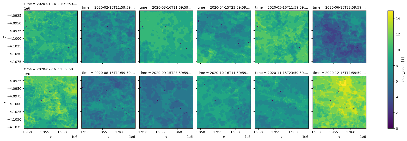
ndvi_anom.clear_count.plot.imshow(col='time', col_wrap=6, cmap="viridis");

Plot NDVI phenology

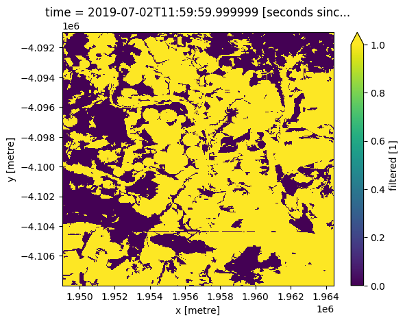
We can use the monthly NDVI to extract the phenology curve for specific landscapes. Limiting our analysis of the area above to a crop mask enables us to investigate the phenology of cropland.

#Load the cropmask dataset for the region

cm = dc.load(product="crop_mask",
             measurements='filtered',
             resampling='nearest',
             like=ndvi_anom.geobox).filtered.squeeze()

cm.plot.imshow(vmin=0, vmax=1);

#Mask the datasets with the crop mask
ndvi_anom_crop = ndvi_anom.where(cm)

Plot phenology curve

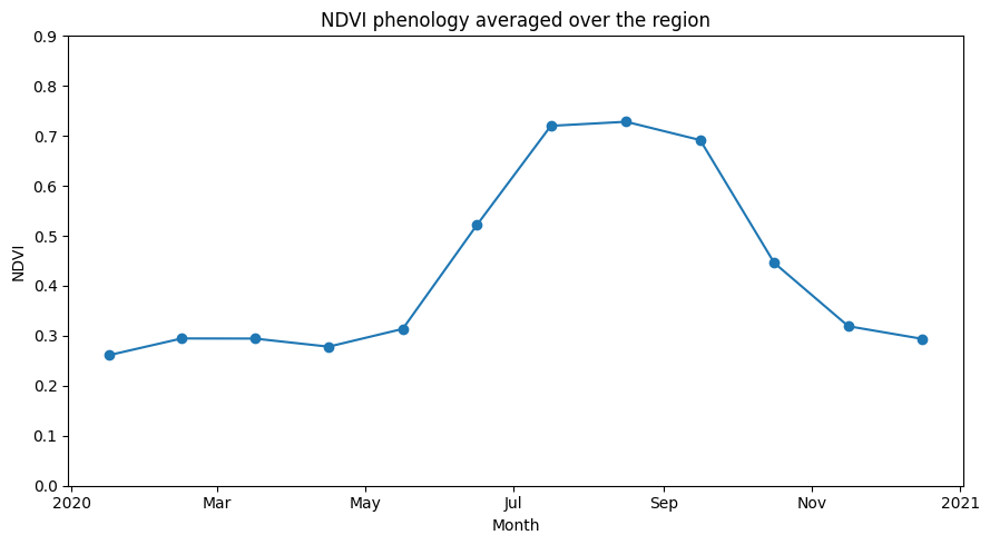
Below, we summarise the datasets spatially by taking the mean across the x and y dimensions. This will leave us with the average trend through time for the region we’ve loaded.

From the phenology plot, we can conclude that crop growth in this area commenced around May and continued until harvest around October.

For a more detailed vegetation phenology analysis, see the notebook Vegetation Phenology notebook.

ndvi_mean_crop = ndvi_anom_crop.ndvi_mean.mean(['x','y'])

ndvi_mean_crop.plot(figsize=(9,5), marker='o')
plt.ylim(0,0.9)
plt.title('NDVI phenology averaged over the region')
plt.xlabel('Month')
plt.ylabel('NDVI')
plt.tight_layout()

Extract NDVI anomalies for a selected month and region

# Select a country
country = "Uganda"

# year and month for anomaly
year_month = "2022-06"

# pixel resolution can got as low as (-30,30) metres,
# but make larger for big areas.
resolution = (-120, 120)

# how to chunk the dataset for use with dask
dask_chunks = dict(x=1000, y=1000)

Load the African Countries shapefile

This shapefile contains polygons for the boundaries of African countries and will allows us to calculate NDVI anomalies within a chosen country.

african_countries = gpd.read_file('../Supplementary_data/Rainfall_anomaly_CHIRPS/african_countries.geojson')

List countries

You can change the country in the analysis parameters cell to any African country. A complete list of countries is printed below.

print(np.unique(african_countries.COUNTRY))

['Algeria' 'Angola' 'Benin' 'Botswana' 'Burkina Faso' 'Burundi' 'Cameroon'
 'Cape Verde' 'Central African Republic' 'Chad' 'Comoros'
 'Congo-Brazzaville' 'Cote d`Ivoire' 'Democratic Republic of Congo'
 'Djibouti' 'Egypt' 'Equatorial Guinea' 'Eritrea' 'Ethiopia' 'Gabon'
 'Gambia' 'Ghana' 'Guinea' 'Guinea-Bissau' 'Kenya' 'Lesotho' 'Liberia'
 'Libya' 'Madagascar' 'Malawi' 'Mali' 'Mauritania' 'Morocco' 'Mozambique'
 'Namibia' 'Niger' 'Nigeria' 'Rwanda' 'Sao Tome and Principe' 'Senegal'
 'Sierra Leone' 'Somalia' 'South Africa' 'Sudan' 'Swaziland' 'Tanzania'
 'Togo' 'Tunisia' 'Uganda' 'Western Sahara' 'Zambia' 'Zimbabwe']

Setup polygon

The country selected needs to be transformed into a geometry object to be used in the load_ard function.

idx = african_countries[african_countries['COUNTRY'] == country].index[0]
geom = Geometry(geom=african_countries.iloc[idx].geometry, crs=african_countries.crs)

Load NDVI anomaly

ndvi_anom = dc.load(
    product="ndvi_anomaly",
    resolution=resolution,
    geopolygon=geom,
    time=year_month,
    dask_chunks=dask_chunks,
).squeeze()

print(ndvi_anom)

<xarray.Dataset> Size: 238MB
Dimensions:           (y: 6070, x: 4364)
Coordinates:
    time              datetime64[ns] 8B 2022-06-15T23:59:59.999999
  * y                 (y) float64 49kB 5.397e+05 5.396e+05 ... -1.886e+05
  * x                 (x) float64 35kB 2.853e+06 2.854e+06 ... 3.377e+06
    spatial_ref       int32 4B 6933
Data variables:
    ndvi_mean         (y, x) float32 106MB dask.array<chunksize=(1000, 1000), meta=np.ndarray>
    ndvi_std_anomaly  (y, x) float32 106MB dask.array<chunksize=(1000, 1000), meta=np.ndarray>
    clear_count       (y, x) int8 26MB dask.array<chunksize=(1000, 1000), meta=np.ndarray>
Attributes:
    crs:           epsg:6933
    grid_mapping:  spatial_ref

african_countries = african_countries.to_crs('epsg:6933')
mask = xr_rasterize(african_countries[african_countries['COUNTRY'] == country], ndvi_anom)

ndvi_anom = ndvi_anom.where(mask==1)

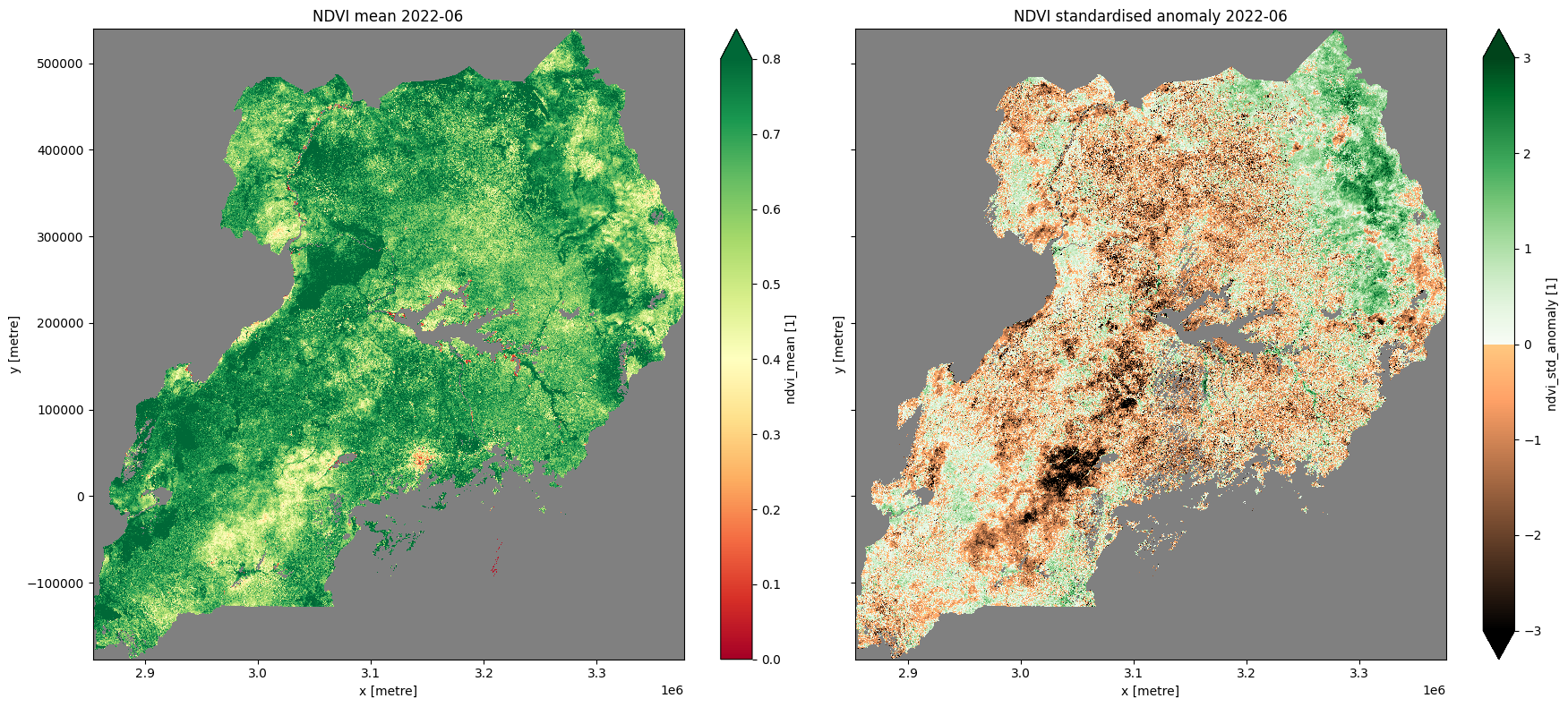
Plot NDVI climatology, monthly mean, and standardised anomaly

# plot all layers
plt.rcParams["axes.facecolor"] = "gray"  # makes transparent pixels obvious
fig, ax = plt.subplots(1, 2, sharey=True, sharex=True, figsize=(18, 8))

ndvi_anom.ndvi_mean.plot.imshow(ax=ax[0], cmap="RdYlGn",vmin=0,vmax=0.8)
ax[0].set_title("NDVI mean " + year_month)

ndvi_anom.ndvi_std_anomaly.plot.imshow(ax=ax[1], cmap=cramp, vmin=-3, vmax=3)
ax[1].set_title("NDVI standardised anomaly " + year_month)
plt.tight_layout();

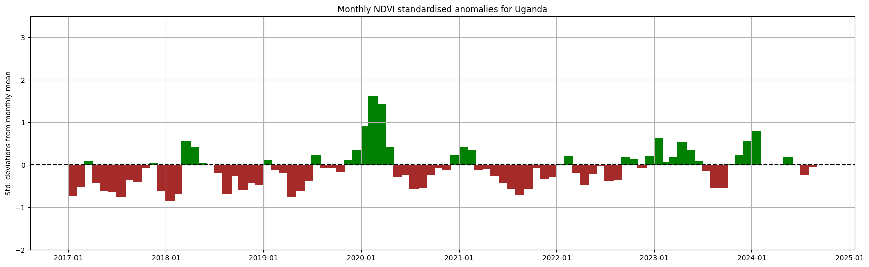
Compare monthly NDVI conditions over the years

ndvi_anom = dc.load(
    product="ndvi_anomaly",
    resolution=resolution,
    geopolygon=geom,
#     time=year_month,
    dask_chunks=dask_chunks,
)

Below, the spatial mean is taken so we can present the monthly anomalies aggregated across the selected country.

spatial_mean_anoms = ndvi_anom.ndvi_std_anomaly.mean(['x','y']).to_dataframe().drop(['spatial_ref'], axis=1)

plt.rcParams["axes.facecolor"] = "white"
fig, ax = plt.subplots(figsize=(21,6))
ax.xaxis.set_major_formatter(mdates.DateFormatter("%Y-%m"))
ax.set_ylim(-2,3.5)
ax.bar(spatial_mean_anoms.index,
       spatial_mean_anoms.ndvi_std_anomaly,
       width=35, align='center',
       color=(spatial_mean_anoms['ndvi_std_anomaly'] > 0).map({True: 'g', False: 'brown'}))
ax.axhline(0, color='black', linestyle='--')
plt.title('Monthly NDVI standardised anomalies for '+ country)
plt.ylabel('Std. deviations from monthly mean');
plt.grid()

---

Additional information

License: The code in this notebook is licensed under the Apache License, Version 2.0. Digital Earth Africa data is licensed under the Creative Commons by Attribution 4.0 license.

Contact: If you need assistance, please post a question on the Open Data Cube Slack channel or on the GIS Stack Exchange using the open-data-cube tag (you can view previously asked questions here). If you would like to report an issue with this notebook, you can file one on Github.

Compatible datacube version:

print(datacube.__version__)

1.8.20

Last Tested:

from datetime import datetime
datetime.today().strftime('%Y-%m-%d')

'2025-01-15'