Sentinel-1 Monthly Mosaic 
Products used: s1_monthly_mosaic
Keywords data used; sentinel-1,:index:datasets; sentinel-1 monthly mosaic, index:SAR
Background
Synthetic Aperture Radar (SAR) sensors have the advantage of operating at wavelengths not impeded by cloud cover and can acquire data over a site during the day or night. The Sentinel-1 mission, part of the Copernicus joint initiative by the European Commission (EC) and the European Space Agency (ESA), provides reliable and repeated wide-area monitoring using its SAR instrument.
The Sentinel-1 monthly mosaics are generated from Radiometric Terrain Corrected (RTC) backscatter data, with variations from changing observation geometries mitigated. In the Monthly Mosaic product, RTC images acquired within a calendar month are combined using a multitemporal compositing algorithm. This algorithm calculates a weighted average of valid pixels, assigning higher weights to pixels with higher local resolution (e.g., slopes facing away from the sensor). This local resolution weighting approach minimizes noise and improves spatial homogeneity in the composites.
More information on how the product is generated can be found in the Copernicus Data Space Ecosystem Documentation.
DE Africa provides access to Sentinel-1 monthly mosaics generated from Interferometric Wide (IW) acquisition mode. The mosaics are organized in a UTM grid with tiles measuring 100 x 100 km and have a spatial resolution of 20 meters.
Description
In this notebook we will load Sentinel-1 Monthly Mosaics.
Topics covered include:
Inspecting the Sentinel-1 monthly mosaics product and measurements available in the datacube
Using the
dc.load()function to load in Sentinel-1 monthly mosaicsVisualising monthly mosaics
Comparing monthly mosaics with monthly NDVI and individual Sentinel-1 scenes ***
Getting started
To run this analysis, run all the cells in the notebook, starting with the “Load packages” cell.
Load packages
[1]:
%matplotlib inline
import datacube
import xarray as xr
import matplotlib.pyplot as plt

from deafrica_tools.plotting import rgb
from deafrica_tools.plotting import display_map
from deafrica_tools.datahandling import mostcommon_crs
from deafrica_tools.bandindices import dualpol_indices
Connect to the datacube
[2]:
dc = datacube.Datacube(app="Sentinel_1_mosaic")
Available products and measurements
List products
We can use datacube’s list_products functionality to inspect DE Africa’s Sentinel-1 products that are available in the datacube. The table below shows the product names that we will use to load the data, a brief description of the data, and the satellite instrument that acquired the data.
[3]:
dc.list_products().loc[dc.list_products()['name'].str.contains('s1')]
[3]:
| name | description | license | default_crs | default_resolution | |
|---|---|---|---|---|---|
| name | |||||
| s1_monthly_mosaic | s1_monthly_mosaic | Monthly Sentinel-1 mosaics of weighted terrain... | None | None | None |
| s1_rtc | s1_rtc | Sentinel 1 Gamma0 normalised radar backscatter | CC-BY-4.0 | EPSG:4326 | (-0.0002, 0.0002) |
[4]:
product = "s1_monthly_mosaic"
List measurements
We can further inspect the data available for each SAR product using datacube’s list_measurements functionality. The table below lists each of the measurements available in the data.
[5]:
measurements = dc.list_measurements()
measurements.loc[product]
[5]:
| name | dtype | units | nodata | aliases | flags_definition | add_offset | scale_factor | |
|---|---|---|---|---|---|---|---|---|
| measurement | ||||||||
| VV | VV | float32 | 1 | NaN | [vv] | NaN | NaN | NaN |
| VH | VH | float32 | 1 | NaN | [vh] | NaN | NaN | NaN |
The Sentinel-1 Monthly Mosaic product has two measurements:
Backscatter in
VVpolarisation, representing weighted average of valid normalizedVVbackscatter values measured over the month.Backscatter in
VHpolarisation, representing weighted average of valid normalizedVHbackscatter values measured over the month.
The two-letter band names indicate the polarization of the light transmitted and received by the satellite. VV refers to the satellite sending out vertically-polarised light and receiving vertically-polarised light back, whereas VH refers to the satellite sending out vertically-polarised light and receiving horizontally-polarised light back.
Load Sentinel-1 Monthly Mosaics using dc.load()
Now that we know what products and measurements are available for the product, we can load data from the datacube using dc.load.
In the example below, we will load Sentinel-1 mosaic for an area around the town of Boma on the Congo River, from April 2023 to March 2024.
We will load data from two polarisation bands,VV and VH. Since the data is provided in UTM grid, we will use the most common projection for the area to load data.
Note: For a more general discussion of how to load data using the datacube, refer to the Introduction to loading data notebook.
[6]:
# Define the area of interest
latitude = -5.87
longitude = 13.06

buffer = 0.05
time = ('2023-04', '2024-03')

bands = ['vv','vh']
[7]:
#add spatio-temporal extent to the query
query = {
    'x': (longitude-buffer, longitude+buffer),
    'y': (latitude+buffer, latitude-buffer),
    'time':time,
}
Visualise the selected area
[8]:
display_map(x=(longitude-buffer, longitude+buffer), y=(latitude+buffer, latitude-buffer))
[8]:
[9]:
output_crs = mostcommon_crs(dc=dc, product=product, query=query)
print(output_crs)
epsg:32733
[10]:
# loading the data
ds_monthly = dc.load(
    product=product,
    measurements=bands,
    output_crs=output_crs,
    resolution=(-20, 20),
    **query
)

print(ds_monthly)
<xarray.Dataset> Size: 22MB
Dimensions:      (time: 9, y: 556, x: 557)
Coordinates:
  * time         (time) datetime64[ns] 72B 2023-05-16T11:59:59.500000 ... 202...
  * y            (y) float64 4kB 9.356e+06 9.356e+06 ... 9.345e+06 9.345e+06
  * x            (x) float64 4kB 2.796e+05 2.797e+05 ... 2.908e+05 2.908e+05
    spatial_ref  int32 4B 32733
Data variables:
    vv           (time, y, x) float32 11MB 0.07513 0.06036 ... 0.1843 0.1746
    vh           (time, y, x) float32 11MB 0.02182 0.02375 ... 0.03499 0.03216
Attributes:
    crs:           epsg:32733
    grid_mapping:  spatial_ref
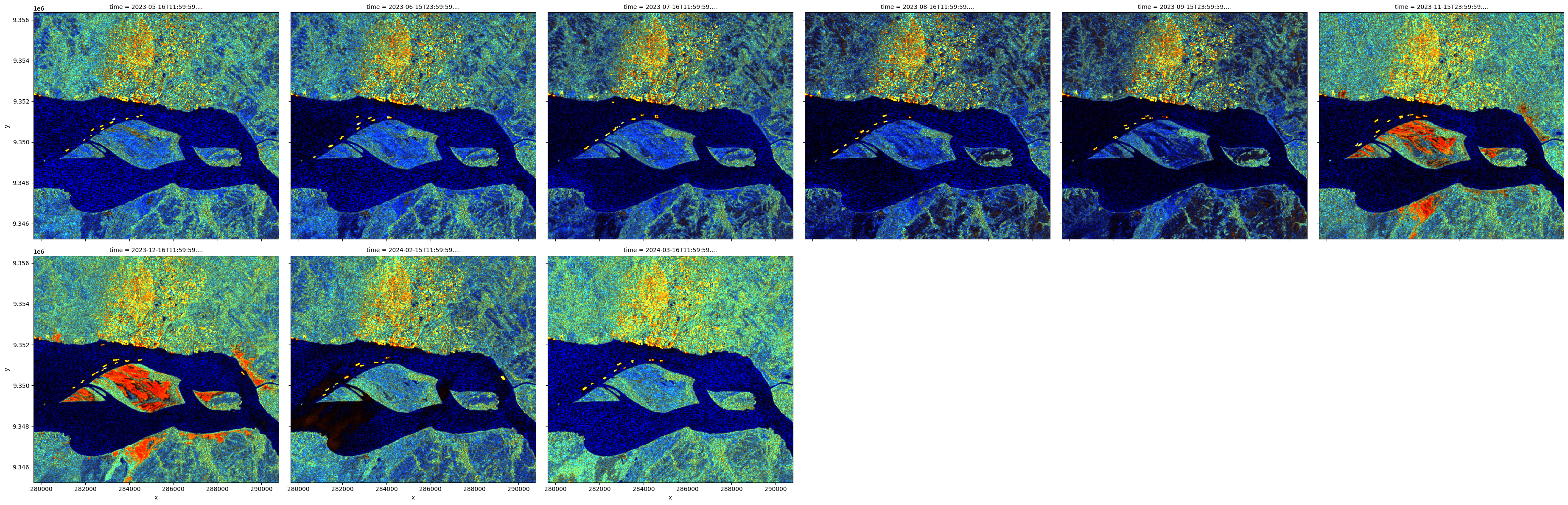
Visualise Sentinel-1 Mosaic
To visualise data from the Sentinel-1 SAR sensor, we calculate the ratio between the vertical and horizontal polarisation bands.
[11]:
# adding a ratio band
ds_monthly['vh_over_vv'] = ds_monthly.vh/ds_monthly.vv
The data is scaled according to the 2nd and 98th percentiles of observations.
[12]:
data_min = ds_monthly.quantile(0.02)
data_max = ds_monthly.quantile(0.98)
[13]:
scaled = (ds_monthly - data_min)/(data_max - data_min)
[14]:
scaled
[14]:
<xarray.Dataset> Size: 67MB
Dimensions:      (time: 9, y: 556, x: 557)
Coordinates:
  * time         (time) datetime64[ns] 72B 2023-05-16T11:59:59.500000 ... 202...
  * y            (y) float64 4kB 9.356e+06 9.356e+06 ... 9.345e+06 9.345e+06
  * x            (x) float64 4kB 2.796e+05 2.797e+05 ... 2.908e+05 2.908e+05
    spatial_ref  int32 4B 32733
    quantile     float64 8B 0.02
Data variables:
    vv           (time, y, x) float64 22MB 0.1371 0.1089 ... 0.3455 0.3271
    vh           (time, y, x) float64 22MB 0.2926 0.319 0.2788 ... 0.4726 0.4339
vh_over_vv (time, y, x) float64 22MB 0.5152 0.7303 ... 0.3057 0.2938The assignment of vertical and horizontal bands as red and green, respectively, and the ratio as the blue band, is a common way to visualise SAR data.
[15]:
rgb(scaled, bands=['vv','vh','vh_over_vv'], col='time', col_wrap=6)
Generate a false colour visualisation
The cell below manipulates the dual-polarisation bands to produce a false colour visualisation based on expected land cover classes given band values. The code is adapted from Markuse, P, shown in Sentinel Hub. The script includes stretch parameter values for various visualisation objectives including ‘redder land’, ‘oil spills’, and ‘bright water’. In this case, we are using the
land_green specification because our area of interest is characterised by dense, green vegetation.
First, functions are defined to produce the visualisation.
[16]:
def sat_enh(rgb_arr, saturation=1.0):
    avg = sum(rgb_arr) / len(rgb_arr)
    return [avg * (1 - saturation) + band * saturation for band in rgb_arr]

def classify_pixel_xr(VV, VH,
                      saturation=1.0,
                      brightness=1.0,
                      water_threshold=25,
                      manual_correction_water=[0.0, 0.0, 0.0],
                      manual_correction_land=[0.0, 0.0, 0.0]):

    def safe_stretch(val, min_val, max_val):
        return ((val - min_val) / (max_val - min_val)).clip(0.0, 1.0)

    water_normal = [
        safe_stretch(VV * 1, 0.0, 0.99),
        safe_stretch(VV * 8, 0.0, 0.99),
        0.5 + VV * 3 + safe_stretch(VH * 2000, 0.0, 0.99)
    ]
    # adjust stretch values to make land greener
    land_green = [
        safe_stretch(VV * 3.0, 0.0, 0.99),
        safe_stretch(VV * 1.4, 0.0, 0.99) + safe_stretch(VH * 8.75, 0.0, 0.99),
        safe_stretch(VH * 1.75, 0.0, 0.99)
    ]

    # Apply manual corrections and brightness
    watervis = [band + corr for band, corr in zip(water_normal, manual_correction_water)]
    landvis = [(band + corr) * brightness for band, corr in zip(land_green, manual_correction_land)]

    # Saturation enhancement
    watervis = sat_enh(watervis, saturation)
    landvis = sat_enh(landvis, saturation)

    # Water mask
    water_mask = (VV / VH) > water_threshold
    result = [xr.where(water_mask, w, l) for w, l in zip(watervis, landvis)]

    # Stack to RGB array
    rgb = xr.concat(result, dim='band')
    rgb = rgb.assign_coords(band=['R', 'G', 'B'])

    return rgb
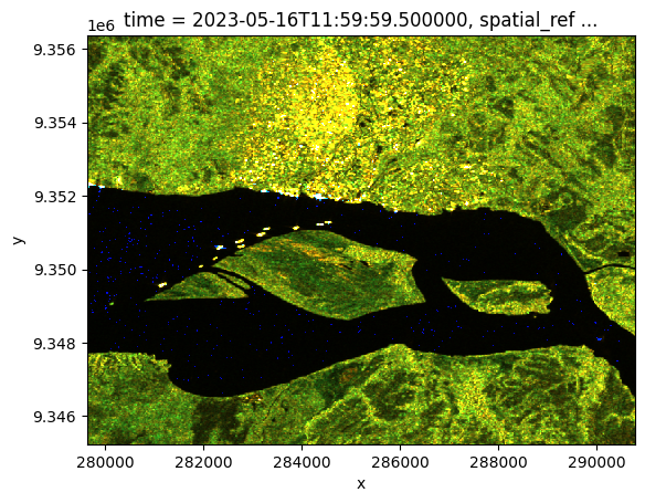
The function is then applied to our Sentinel-1 monthly dataset and the result plotted. We can see urban areas, vegetation, and water in an enhanced ‘false colour’.
[17]:
false_col = classify_pixel_xr(ds_monthly.vv, ds_monthly.vh).isel(time=0)
false_col.plot.imshow()
Clipping input data to the valid range for imshow with RGB data ([0..1] for floats or [0..255] for integers). Got range [0.000113667695..298.3589].
[17]:
<matplotlib.image.AxesImage at 0x7f4ff403a4b0>
Advantages of using the monthly mosaics
The regular monthly spacing enables easy time series analysis, either alone or combined with other datasets.
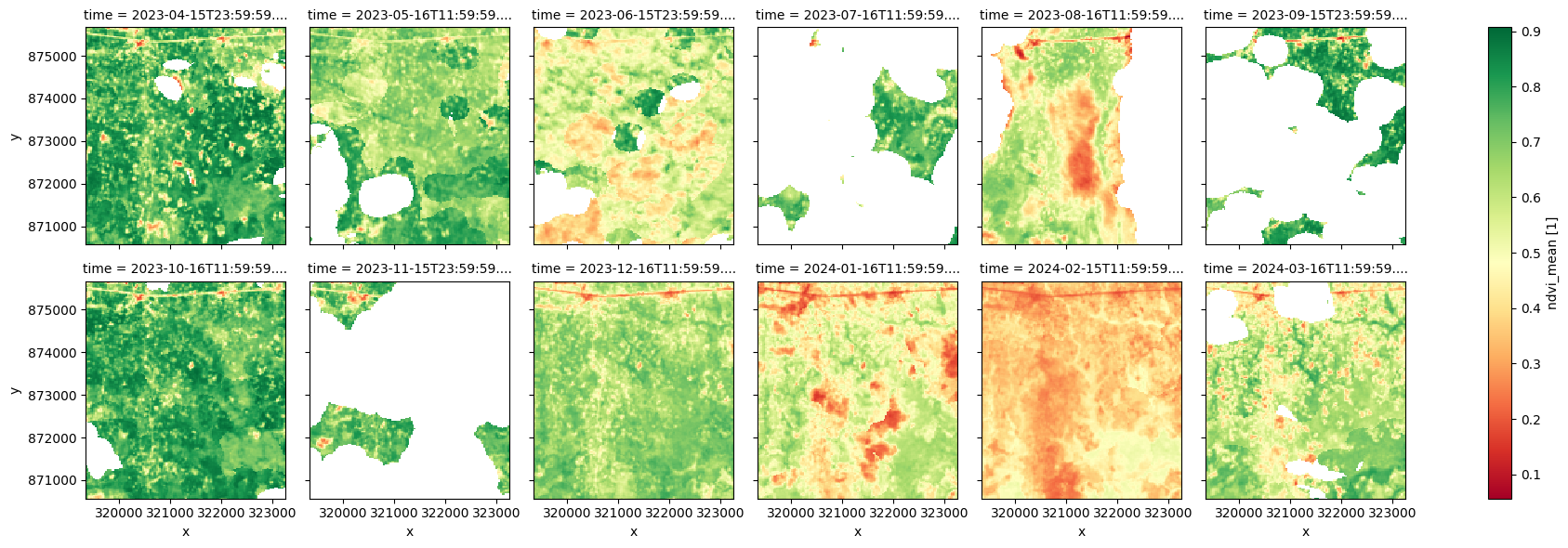
Over cloudy regions like the example area in Southwestern Nigeria, radar mosaics provide a reliable means of tracking changes throughout the year, particularly during the rainy season when crops are actively growing.
Below, we compare radar mosaics to monthly NDVI measurements. In much of this region, NDVI data is either unavailable in certain months (e.g., July, September, November) due to persistent cloud cover or affected by residual clouds that were not correctly filtered out (e.g., June, August). This leads to an inaccurate representation of the growing trends, as shown in the plot below.
In contrast, radar data remains unaffected by cloud cover and successfully tracks crop development throughout the entire year, providing a more consistent and reliable dataset for monitoring agricultural changes.
In areas less affected by clouds, radar can provide complementary information to optical data, enhancing the overall monitoring capabilities.
[18]:
# Define the area of interest
latitude = 6.86
longitude = 3.33

buffer = 0.02

#add spatio-temporal extent to the query
query = {
    'x': (longitude-buffer, longitude+buffer),
    'y': (latitude+buffer, latitude-buffer),
    'time':time,
}
The next area of interest is near Lagos, Nigeria. It is mostly agricultural land with a major road running east-west in the very north of the area.
[19]:
display_map(x=(longitude-buffer, longitude+buffer), y=(latitude+buffer, latitude-buffer))
[19]:
[20]:
# loading the monthly NDVI data
ds_monthly = dc.load(
    product=product,
    measurements=bands,
    output_crs=output_crs,
    resolution=(-20, 20),
    **query
)

print(ds_monthly)
<xarray.Dataset> Size: 4MB
Dimensions:      (time: 10, y: 232, x: 232)
Coordinates:
  * time         (time) datetime64[ns] 80B 2023-05-16T11:59:59.500000 ... 202...
  * y            (y) float64 2kB 1.078e+07 1.078e+07 ... 1.077e+07 1.077e+07
  * x            (x) float64 2kB -8.005e+05 -8.004e+05 ... -7.959e+05 -7.958e+05
    spatial_ref  int32 4B 32733
Data variables:
    vv           (time, y, x) float32 2MB 0.159 0.1662 0.1793 ... 0.2324 0.2076
    vh           (time, y, x) float32 2MB 0.04548 0.04205 ... 0.04563 0.05365
Attributes:
    crs:           epsg:32733
    grid_mapping:  spatial_ref
[21]:
# load monthly mean NDVI from the NDVI anomaly product

ndvi_anom = dc.load(
    product="ndvi_anomaly",
    measurements=["ndvi_mean"],
    **query,
)
[22]:
# visualise monthly NDVI

ndvi_anom.ndvi_mean.plot.imshow(col='time', col_wrap=6, cmap="RdYlGn");
In this case, we’ll calculate the Radar Vegetation Index (RVI) which is one of the dual-polarisation indices available in the DE Africa tools package.
[23]:
# Calculate the chosen radar vegetation index and add it to the loaded data set

ds_monthly = dualpol_indices(ds_monthly, index='RVI')
[24]:
# Compare monthly NDVI trend and radar measured vegetation trend

fig, ax1 = plt.subplots(figsize=(11,4))
ndvi_anom.ndvi_mean.mean(['x','y']).isel(time=ndvi_anom.ndvi_mean.isnull().mean(['x','y'])<0.5).plot.line('b:^', ax=ax1, label='NDVI');
ax1.set_title('');
plt.legend(loc='lower left');

# Create a second y-axis
ax2 = ax1.twinx()
ds_monthly.RVI.mean(['x', 'y']).plot.line('r:^', ax=ax2, label='RVI');
ax2.set_title('');

plt.legend(loc='upper right');
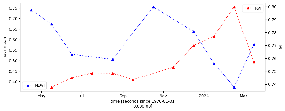
The NDVI trend above is unreliable due to missing data and the presence of residual clouds, particularly during the rainy season. We can also see some months are missing from the NDVI timeseries.
Comparison to individual Sentinel-1 scenes
Monthly mosaics offer reduced noise (as shown below) and improved spatial homogeneity compared to individual Sentinel-1 scenes.
[25]:
# reduce the time window to one month for this demonstration
query['time'] = ('2023-04')

# loading individual Sentinel-1 scenes
ds_S1 = dc.load(product='s1_rtc',
                measurements=bands + ['mask', 'area'],
                group_by="solar_day",
                output_crs = ds_monthly.attrs['crs'], resolution = (-20,20),
                **query)

print(ds_S1)
<xarray.Dataset> Size: 4MB
Dimensions:      (time: 5, y: 232, x: 232)
Coordinates:
  * time         (time) datetime64[ns] 40B 2023-04-04T05:30:28.075105 ... 202...
  * y            (y) float64 2kB 1.078e+07 1.078e+07 ... 1.077e+07 1.077e+07
  * x            (x) float64 2kB -8.005e+05 -8.004e+05 ... -7.959e+05 -7.958e+05
    spatial_ref  int32 4B 32733
Data variables:
    vv           (time, y, x) float32 1MB 0.1334 0.1753 0.1383 ... 0.1928 0.1374
    vh           (time, y, x) float32 1MB 0.03488 0.03196 ... 0.05957 0.08005
    mask         (time, y, x) uint8 269kB 1 1 1 1 1 1 1 1 1 ... 1 1 1 1 1 1 1 1
    area         (time, y, x) float32 1MB 1.015 1.031 1.019 ... 1.016 1.041
Attributes:
    crs:           epsg:32733
    grid_mapping:  spatial_ref
[26]:
fig, (ax1, ax2) = plt.subplots(1, 2, figsize=(8,4))

# Plot individual Sentinel-1 observation
ds_S1.vh.isel(time=0).plot.imshow(robust=True, ax=ax1)

# monthly mosaic
ds_monthly.isel(time=0).vh.plot.imshow(robust=True, ax=ax2)

# title
ax1.set_title('S1 RTC scene')
ax2.set_title('S1 Monthly Mosaic')
[26]:
Text(0.5, 1.0, 'S1 Monthly Mosaic')
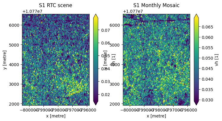
With reduced noise, small features are more visible in the monthly mosaic, notably the major road/highway in the northern part of the area of interest.
Other considerations
Combining acquisitions from different orbit directions and look angles helps reduce radar shadow effects in mosaics. However, in steep terrain, some areas may consistently fall into radar shadow, making reliable backscatter measurements impossible. These regions are marked as NaN in the mosaic.
When high temporal resolution is crucial, individual Sentinel-1 scenes offer greater flexibility for analysis.
Additionally, a local resolution weighting approach can be applied to combine Sentinel-1 scenes from different time periods. For slow-changing landscapes, a time window longer than a month can be used to futher reduce noise.
Generating weighted mosaic
[27]:
# apply local resolution weighting to generate a mosaic

weight = 1 / ds_S1.area.where(ds_S1.mask==1)
ds_S1_weighted = (ds_S1[['vv', 'vh']].where(ds_S1.mask==1)*weight/weight.sum(dim='time')).sum(dim='time')
[28]:
ds_S1_weighted.vh.plot.imshow(robust=True);
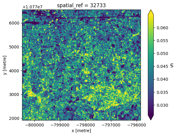
The mosaic generated above differs slightly from the monthly mosaic product due to variations in projection and resampling methods used during processing.
Additional information
License: The code in this notebook is licensed under the Apache License, Version 2.0. Digital Earth Africa data is licensed under the Creative Commons by Attribution 4.0 license.
Contact: If you need assistance, please post a question on the Open Data Cube Slack channel or on the GIS Stack Exchange using the open-data-cube tag (you can view previously asked questions here). If you would like to report an issue with this notebook, you can file one on
Github.
Compatible datacube version:
[29]:
print(datacube.__version__)
1.8.20
Last Tested:
[30]:
from datetime import datetime
datetime.today().strftime('%Y-%m-%d')
[30]:
'2025-04-07'