Mountain Green Cover Index Notebook (SDG 15.4.2)

Disclaimer: The notebook is work in progress. This workshop will be a good forum to get feedback to refine the notebook. Thank you.

Background

Sustainable Development Goal 15:

Protect, restore and promote sustainable use of terrestrial ecosystems, sustainably manage forests, combat desertification, and halt and reverse land degradation and halt biodiversity loss.

Target 15.4

By 2030, ensure the conservation of mountain ecosystems, including their biodiversity, in order to enhance their capacity to provide benefits that are essential for sustainable development.

Indicator 15.4.2: Mountain Green Cover Index

The Mountain Green Cover Index (MGCI) is designed to measure the extent and the changes of green vegetation in mountain areas - i.e. forest, shrubs, trees, pasture land, crop land, etc. – in order to monitor progress towards the mountain target. MGCI is defined as the percentage of green cover over the total surface of the mountain region of a given country and for a given reporting year. The aim of the index is to monitor the evolution of the green cover and thus assess the status of conservation of mountain ecosystems. More information on MGCI can be found here.

Description

The methodology to calculate the Mountain Green Cover index was initially developed by FAO (De Simone et al., 2021).

The Mountain Green Cover index is calculated using two descriptor layers of information:

1. A mountain descriptor layer: mountains can be defined with reference to a variety of parameters, such as climate, elevation, ecology (Körner et al., 2011) (Karagulle et al., 2017). This methodology adheres to the UNEP- WCMC mountain definition, relying in turn on the mountain description proposed by Kapos et al. (2000).

2. A vegetation descriptor layer: The vegetation descriptor layer categorizes land cover into green and non-green areas. Green vegetation includes both natural vegetation and vegetation resulting from anthropic activity (e.g. crops, afforestation, etc.). Non-green areas include very sparsely vegetated areas, bare land, water, permanent ice/snow and urban areas. The vegetation description layer can be derived in different ways, but remote sensing based land cover maps are the most convenient data source for this purpose, as they provide the required information on green and non-green areas in a spatially explicit manner and allow for comparison over time through land cover change analysis.

Currently, FAO uses the land cover time series produced by the European Space Agency (ESA) under the Climate Change Initiative (CCI) as a general solution. More information is provided here.

The notebook does the following:

1. Calculate the Kapos Mountain Range class for the study area

2. Reclassify ESA CCI to IPCC Classification and Green and Non Green

3. Generate the Mountain Green Cover Index (MGCI)

---

Getting started

To run this analysis, run all the cells in the notebook, starting with the “Load packages” cell.

Load packages

%matplotlib inline

import os
import datacube
import matplotlib.pyplot as plt
import xarray as xr
import numpy as np
import geopandas as gpd
import pandas as pd
from scipy.ndimage import uniform_filter, maximum_filter, minimum_filter
from odc.geo.xr import write_cog
from odc.geo.geom import Geometry
from odc.geo.crs import CRS

from deafrica_tools.datahandling import load_ard
from deafrica_tools.plotting import rgb, display_map, plot_lulc, map_shapefile
from deafrica_tools.bandindices import calculate_indices
from deafrica_tools.dask import create_local_dask_cluster
from deafrica_tools.spatial import xr_rasterize

from odc.algo import xr_reproject

Set up a Dask cluster

Dask can be used to better manage memory use and conduct the analysis in parallel. For an introduction to using Dask with Digital Earth Africa, see the Dask notebook.

Note: We recommend opening the Dask processing window to view the different computations that are being executed; to do this, see the Dask dashboard in DE Africa section of the Dask notebook.

To use Dask, set up the local computing cluster using the cell below.

create_local_dask_cluster()

Client

Client-d1c4039c-d439-11ef-a88b-1e01ca941b00

Connection method: Cluster object	Cluster type: distributed.LocalCluster
Dashboard: /user/victoria@kartoza.com/proxy/8787/status

Launch dashboard in JupyterLab

Cluster Info

LocalCluster

c94f3bda

Dashboard: /user/victoria@kartoza.com/proxy/8787/status	Workers: 1
Total threads: 7	Total memory: 59.21 GiB
Status: running	Using processes: True

Scheduler Info

Scheduler

Scheduler-b7897c02-61c0-44de-b4af-80cbb1a2a1a9

Comm: tcp://127.0.0.1:38483	Workers: 1
Dashboard: /user/victoria@kartoza.com/proxy/8787/status	Total threads: 7
Started: Just now	Total memory: 59.21 GiB

Workers

Worker: 0

Comm: tcp://127.0.0.1:45405	Total threads: 7
Dashboard: /user/victoria@kartoza.com/proxy/40257/status	Memory: 59.21 GiB
Nanny: tcp://127.0.0.1:43199
Local directory: /tmp/dask-scratch-space/worker-9s61qbw2

Analysis parameters

The following cell sets important parameters for the analysis:

• time : This is the time period of interest for the analysis.

• output_crs : The coordinate reference system that the loaded data is to be reprojected to.

• dask_chunks : the size of the dask chunks, dask breaks data into manageable chunks that can be easily stored in memory.

• output_dir : The directory in which to store results from the analysis.

time = 2019

output_crs = "EPSG:6933"

dask_chunks = {"time": 1, "x": 3000, "y": 3000}

# Create the output directory to store the results.
output_dir = "results"
os.makedirs(output_dir, exist_ok=True)

Connect to the datacube

Connect to the datacube so we can access DE Africa data. The app parameter is a unique name for the analysis which is based on the notebook file name.

dc = datacube.Datacube(app="mgci")

Select a country

Load the African Countries GeoJSON. This file contains polygons for the boundaries of African countries.

african_countries  = gpd.read_file("../../Supplementary_data/MGCI/african_countries.geojson")
african_countries.explore()

Make this Notebook Trusted to load map: File -> Trust Notebook

List the countries in the African Countries GeoJSON.

np.unique(african_countries["COUNTRY"])

array(['Algeria', 'Angola', 'Benin', 'Botswana', 'Burkina Faso',
       'Burundi', 'Cameroon', 'Cape Verde', 'Central African Republic',
       'Chad', 'Comoros', 'Congo-Brazzaville', 'Cote d`Ivoire',
       'Democratic Republic of Congo', 'Djibouti', 'Egypt',
       'Equatorial Guinea', 'Eritrea', 'Ethiopia', 'Gabon', 'Gambia',
       'Ghana', 'Guinea', 'Guinea-Bissau', 'Kenya', 'Lesotho', 'Liberia',
       'Libya', 'Madagascar', 'Malawi', 'Mali', 'Mauritania', 'Morocco',
       'Mozambique', 'Namibia', 'Niger', 'Nigeria', 'Rwanda',
       'Sao Tome and Principe', 'Senegal', 'Sierra Leone', 'Somalia',
       'South Africa', 'Sudan', 'Swaziland', 'Tanzania', 'Togo',
       'Tunisia', 'Uganda', 'Western Sahara', 'Zambia', 'Zimbabwe'],
      dtype=object)

From the countries above, you can choose any and type it at the country variable below.

country = "Rwanda"

idx = african_countries[african_countries['COUNTRY'] == country].index[0]
geom = Geometry(geom=african_countries.iloc[idx].geometry, crs=african_countries.crs)

# Set up daatcube query object.
query = {
    "geopolygon": geom,
    "output_crs": output_crs,
    "dask_chunks": dask_chunks,
}

Load SRTM DEM dataset at 1000m resolution

ds = dc.load(product="dem_srtm",
             resolution=(-1000, 1000),
             measurements="elevation",
             **query)

### Neighborhood reduction operation

# Implmenting the reducers on the dem results
# var ler = dem.reduceNeighborhood({reducer: ee.Reducer.minMax(),
# kernel: ee.Kernel.circle({radius:7000, units:’meter’})});
def reduce_nei(da, size, pre):
    img = da.values
    if pre == "max":
        img = maximum_filter(img, size=size, mode="nearest")
    else:
        img = minimum_filter(img, size=size, mode="nearest")

    return img


ds_max = ds.elevation.groupby("time").apply(reduce_nei, size=7, pre="max")
ds_min = ds.elevation.groupby("time").apply(reduce_nei, size=7, pre="min")

Calculating the local elevation range (LER)

ds["ler_range"] = ds_max - ds_min

Load SRTM DEM slope derivative dataset at 30m resolution

ds_slope = dc.load(product="dem_srtm_deriv",
                   resolution=(-30, 30),
                   measurements="slope",
                   **query)

# Mask using the country polygon.
african_countries = african_countries.to_crs(output_crs)
mask = xr_rasterize(african_countries[african_countries['COUNTRY'] == country],  ds_slope)
ds_slope = ds_slope.where(mask)

Upsampling dem_strm dataset at 1000m to 30m resolution

ds = xr_reproject(src=ds, geobox=ds_slope.geobox, resampling="nearest")

# Mask using the country polygon.
ds = ds.where(mask)

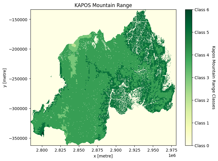
Generating Kapos range mountain classes

classess = [0, 1, 2, 3, 4, 5, 6]
class_label = ["Class 0", "Class 1", "Class 2", "Class 3", "Class 4", "Class 5", "Class 6"]

elevation = ds["elevation"]
slope = ds_slope["slope"]
ler_range = ds["ler_range"]

conditions = [(elevation < 300),
              (elevation > 4500),
              (elevation >= 3500) & (elevation < 4500),
              (elevation >= 2500) & (elevation < 3500),
              (elevation >= 1500) & (elevation < 2500) & (slope > 2),
              (elevation >= 1000) & (elevation < 1500) & ((slope > 5) | (ler_range > 300)),
              (elevation >= 300) & (elevation < 1000) & (ler_range > 300)]

ds["kapo_class"] = xr.DataArray(np.select(conditions, classess),
                                coords={"time": ds.time, "y": ds.y, "x": ds.x},
                                dims=["time", "y", "x"]).astype("int8")

/opt/venv/lib/python3.12/site-packages/distributed/client.py:3361: UserWarning: Sending large graph of size 382.93 MiB.
This may cause some slowdown.
Consider loading the data with Dask directly
 or using futures or delayed objects to embed the data into the graph without repetition.
See also https://docs.dask.org/en/stable/best-practices.html#load-data-with-dask for more information.
  warnings.warn(
/opt/venv/lib/python3.12/site-packages/distributed/client.py:3361: UserWarning: Sending large graph of size 382.94 MiB.
This may cause some slowdown.
Consider loading the data with Dask directly
 or using futures or delayed objects to embed the data into the graph without repetition.
See also https://docs.dask.org/en/stable/best-practices.html#load-data-with-dask for more information.
  warnings.warn(
/opt/venv/lib/python3.12/site-packages/distributed/client.py:3361: UserWarning: Sending large graph of size 383.26 MiB.
This may cause some slowdown.
Consider loading the data with Dask directly
 or using futures or delayed objects to embed the data into the graph without repetition.
See also https://docs.dask.org/en/stable/best-practices.html#load-data-with-dask for more information.
  warnings.warn(
/opt/venv/lib/python3.12/site-packages/distributed/client.py:3361: UserWarning: Sending large graph of size 430.82 MiB.
This may cause some slowdown.
Consider loading the data with Dask directly
 or using futures or delayed objects to embed the data into the graph without repetition.
See also https://docs.dask.org/en/stable/best-practices.html#load-data-with-dask for more information.
  warnings.warn(

Plotting the Kapos Mountain range classes

kap = ds["kapo_class"].plot(size=6, add_colorbar=False, cmap="YlGn")
kap_c = plt.colorbar(kap)
kap_c.set_ticks(classess)
kap_c.set_ticklabels(class_label)
kap_c.set_label("Kapos Mountain Range Classes", loc="center", labelpad=15, rotation=270)
plt.title("KAPOS Mountain Range")
plt.savefig(f"results/kapos_{country}")
plt.show()

Loading ESA Climate Change Initiative Land Cover dataset at 300m resolution

# load the data.
ds_cci = dc.load(product="cci_landcover",
                 time=(f'{time-9}', f'{time}'),
                 measurements="classification",
                 resolution=(-300, 300),
                 **query)

# Mask the dataset to the country polygon.
mask = xr_rasterize(african_countries[african_countries['COUNTRY'] == country], ds_cci)
ds_cci = ds_cci.where(mask)

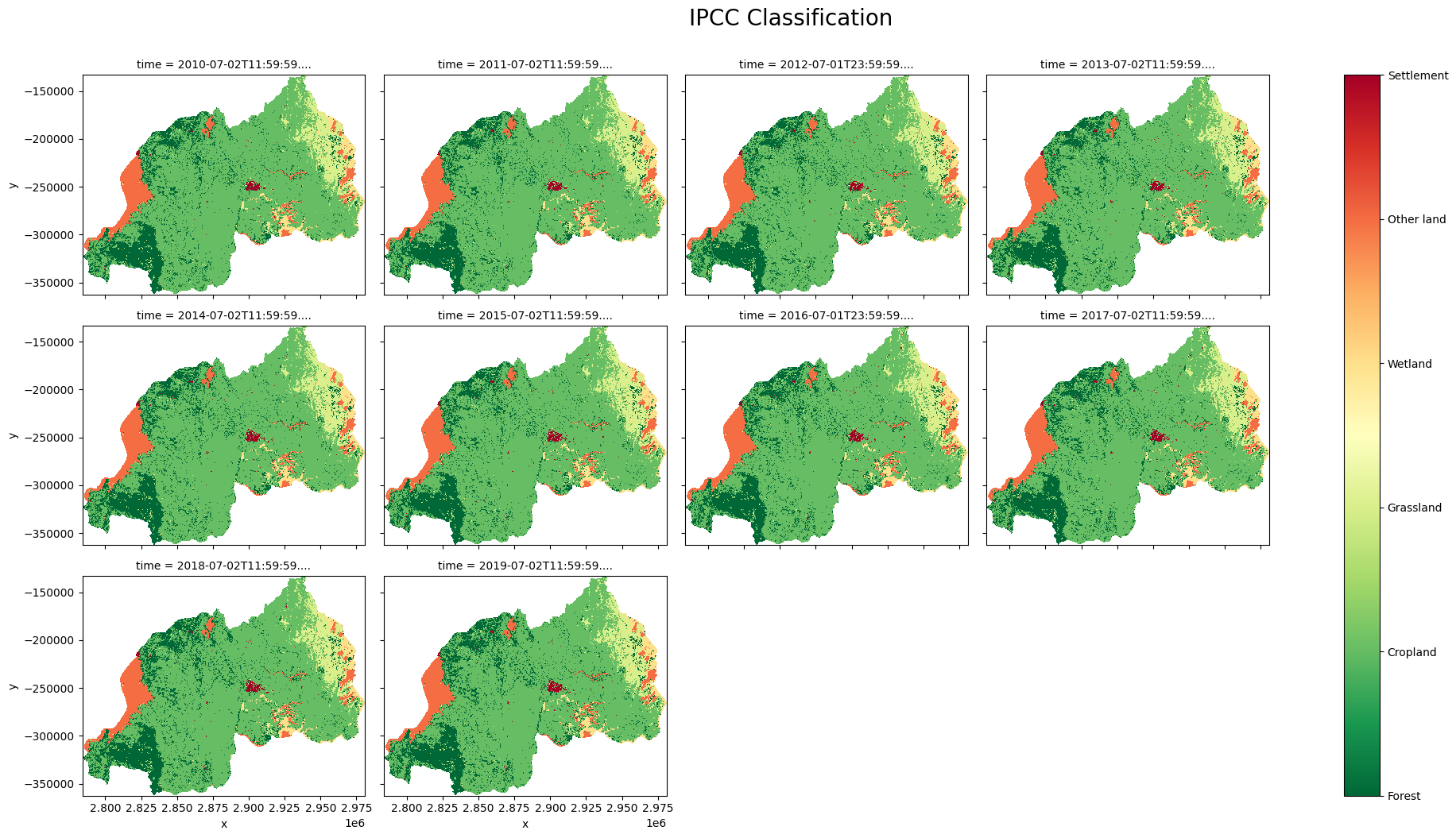
Reclassify CCI land Cover to IPCC Land Cover Classes

ipcc_classess = ['Forest', 'Cropland', 'Grassland', 'Wetland', 'Other land', 'Settlement']
ipcc_classess_num = [1, 2, 3, 4, 5, 6]

ds_clas = ds_cci['classification']
#IPCC Classification
forest = [50, 60, 61, 62, 70, 71, 72, 80, 81, 82, 90, 100]
cropland = [10, 11, 12, 20, 30, 110]
grassland = [40, 120, 121, 122, 130, 140]
wetland = [160, 170, 180]
otherland = [150, 151, 152, 153, 200, 201, 202, 210, 220]
settlement = [190]

ipcc_condition = [ds_clas.isin(forest),
                  ds_clas.isin(cropland),
                  ds_clas.isin(grassland),
                  ds_clas.isin(wetland),
                  ds_clas.isin(otherland),
                  ds_clas.isin(settlement)]

ds_cci["ipcc_classification"] = xr.DataArray(np.select(ipcc_condition, ipcc_classess_num),
                                             coords={"time": ds_cci.time, "y": ds_cci.y, "x": ds_cci.x},
                                             dims=["time", "y", "x"]).astype("int8").where(mask)

Plotting IPCC Classification

clas = ds_cci["ipcc_classification"].plot(col='time',
                                          add_colorbar=False,
                                          figsize = (20, 10),
                                          cmap="RdYlGn_r",
                                          col_wrap = 4)

clas.fig.suptitle("IPCC Classification", ha="center", y=1.05, size=20)
clasp = plt.colorbar(clas._mappables[-1], ax = clas.axs)
clasp.set_ticks(ipcc_classess_num)
clasp.set_ticklabels(ipcc_classess)
plt.savefig(f"results/IPCC_{country}")
plt.show()

Reclassify IPCC Classification to Green and Non Green Classes

gng_classess = ["Green", "Non Green"]
gng_classess_num = [1, 2]
recl_condition = [ds_cci["ipcc_classification"].isin([1, 2, 3, 4]),
                  ds_cci["ipcc_classification"].isin([5, 6])]

ds_cci["green_non_green"] = xr.DataArray(np.select(recl_condition, gng_classess_num),
                                         coords={"time": ds_cci.time, "y": ds_cci.y, "x": ds_cci.x},
                                         dims=["time", "y", "x"]).astype("int8").where(mask)

Plotting Green/Non Green Classification

gng = ds_cci["green_non_green"].plot(col='time',
                                     add_colorbar=False,
                                     figsize = (20, 10),
                                     cmap="RdYlGn_r",
                                     col_wrap = 4)


gng.fig.suptitle("Green and Non-Green Classification", ha="center", y=1.05, size=20)
gngp = plt.colorbar(gng._mappables[-1], ax = gng.axs)
gngp.set_ticks(gng_classess_num)
gngp.set_ticklabels(gng_classess)
plt.savefig(f"results/Green_Non_Green_{country}")
plt.show()

Downsampling dem_strm dataset at 30m to 300m resolution

ds = (xr_reproject(src=ds, geobox=ds_cci.geobox)).squeeze()

## Pixel Area Conversion

pixel_length = 300  # in metres
m_per_km = 1000  # conversion from metres to kilometres
area_per_pixel = pixel_length ** 2 / m_per_km ** 2

Calculating the Mountain Green Cover Index (MGCI)

mgci = {}
years_int=[y[0] for y in ds_cci.groupby('time.year')]
mountain_indices = [y[0] for y in ds.groupby("kapo_class")][1:]

# Mountain Green Cover Area = sum of mountain area (Km2) covered by cropland,
# grassland, forestland, shrubland, and wetland, as defined based on the IPCC classification;
ipcc_green = (ds["kapo_class"].where(ds_cci["ipcc_classification"].isin([1, 2, 3, 4]), np.nan)).astype("int8")

for mountain_index in mountain_indices:
    # Mountain Green Cover Area (Numerator)
    numerator = ipcc_green.where(
        ds['kapo_class'] == mountain_index).sum(dim=["x", "y"])  * area_per_pixel
    # Total Mountain Area = total area (Km2) of mountains. In both the numerator and
    # denominator, Mountain is defined according to Kapos et al. in 2000
    total_mountain_area = ds["kapo_class"].where(
        ds['kapo_class'] == mountain_index).sum(dim=["x", "y"]) * area_per_pixel
    mgci[mountain_index] = (numerator.values / total_mountain_area.values) * 100
mgci = pd.DataFrame.from_dict(mgci, orient="index", columns = years_int)

mgci = mgci.round(2)

Plotting Mountain Green Cover Index

for n in range(len(mgci)):
    mgci.iloc[n].plot(kind="line", figsize=(15,5), marker='o')

plt.title(f"Mountain Green Cover Index for {country}")
plt.legend(loc='center right', bbox_to_anchor=(1.13, 0.25), title="Kapos Mountain \n Range Classes")
plt.xlabel("Year")
plt.ylabel("MGCI Percentage")
plt.xticks(rotation=0)
plt.grid()
plt.savefig(f"results/MGCI_{country}")
plt.show()

---

Additional information

License: The code in this notebook is licensed under the Apache License, Version 2.0. Digital Earth Africa data is licensed under the Creative Commons by Attribution 4.0 license.

Contact: If you need assistance, please post a question on the Open Data Cube Slack channel or on the GIS Stack Exchange using the open-data-cube tag (you can view previously asked questions here). If you would like to report an issue with this notebook, you can file one on Github.

Compatible datacube version:

print(datacube.__version__)

Last Tested:

from datetime import datetime
datetime.today().strftime('%Y-%m-%d')